


Abstract
Purpose: The range precision in carbon ion therapy is extremely sensitive to tissue density variations. A high energy carbon beam, after crossing a high-gradient edge parallel to the beam direction, suffers from range mixing leading to the detection of multiple Bragg peaks (BPs) varying intensity and water equivalent thickness (WET). The purpose of this work was to introduce a model that determines the position of a high-gradient edge based on information acquired from carbon transmission imaging. Methods: A model was derived to determine the lateral distance between the irradiation beam propagation axis and the edge position. To validate it, carbon beams were simulated and propagated through two parametric phantoms: (1) a bone cube in a water tank and (2) a semi-cylindrical bone insert in a water tank. The method was tested in a lung tumor case where range mixing led to more than two BPs being detected, requiring an iterative BP decomposition to determine the fraction of carbon ions crossing the materials surrounding the edge of interest. Results: The theoretical model predicted the edge position relative to the beam position with an error ≤1 mm for all studied cases with a maximum dose delivered of 24 μGy. Conclusions: The method presented here is a proof of principle. It does not take into account clinical uncertainties. However, this approach provided promising results suggesting that future extension to assess the impact of clinical uncertainties should be performed.
Export citation and abstract BibTeX RIS
1. Introduction
The limited range of carbon ions represents one of the main reasons why these are used in cancer therapy. An energetic carbon ion beam presents an increased stopping power towards its finite range, the so called Bragg peak (BP). The range of a charged particle depends on different tissue properties, such as density, atomic composition and ionization potential. In a clinical environment, carbon ions are delivered using a pencil beam that has a lateral Gaussian distribution around the mean position. Hence, carbon ions from the same incident beam, may traverse various materials with different tissue properties and consequently have different ranges. This effect is further emphasized within the lung region where a large difference between the tumor density (about 0.9 gcm−3) and the lung tissue (between 0.3–0.45 gcm−3) can be observed. As documented by Mori et al [1, 2], tumor shifts/shrinkage can lead to geographical miss and/or high dose deposition in organs at risk (OARs).
Different approaches have been considered to account for these effects [1]. One of these approaches is carbon ion imaging, which offers direct information about the carbon ion beam range [3–8]. Recent detectors [3, 6] have been developed with the aim to reproduce carbon ion radiography/Computed Tomography (CT). Due to the high level of secondaries produced by carbon ions when interacting with matter, imaging with these particles is done with range detectors rather than energy detectors. Range detectors measure the depth-energy deposition curve of carbon ions after crossing the materials to be imaged. The BP position of the obtained signal in the range detector is related to the energy loss of the carbon ions. However, as stated earlier, carbon ions from the same beam can have different ranges. In a range detector, carbon ions with different ranges create a depth-energy distribution containing multiple BPs. Krah et al [9] proposed an imaging processing method that approximates the signal as a superposition of individual Bragg curves with varying exit energies.
In this work, a theoretical method is proposed to measure the edge position of a tumor using a concept similar to the one proposed by Krah et al [9]. The method requires a pencil beam crossing a patient, interacting with a high-gradient edge. The pencil must also have a sufficiently high energy to cross the the phantom and be measured in a distal range detector. Then, the position of the tumour edge (generally related to the gross tumor volume) is inferred from the intensity of the BPs recorded. A sizable advantage of this model is that it yields precise tumor position for a very low dose to the patient since a minimum number irradiation spots are necessary.
2. Materials and methods
A novel theoretical model to calculate the position of high-gradient edges is presented. A general equation was derived (section 2.1) to calculate the lateral distance, denoted Y, between the central position of a carbon ion beam and a high-gradient edge (figure 1). In section 2.2, the formalism was extended to multiple high-gradient edges and in section 2.4 the model was used to determine tumor edges in a patient with lung cancer. Parametric and voxelized phantoms were simulated using Monte Carlo (MC) algorithms to validate the model.
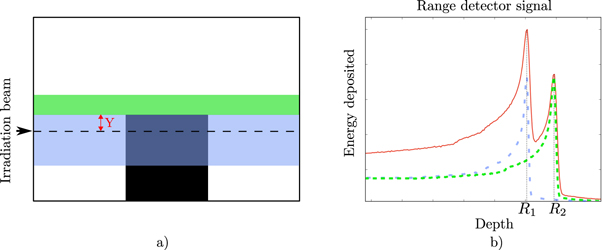
Figure 1. Figure (a) the black square represents a bone insert placed in a water volume. The green shaded area represents the carbon ions that cross the least dense material, whilst the blue shaded area represents the carbon ions crossing the densest material. Figure (b) shows the detected signal from irradiating the phantom (red line). The total signal is the summation of all Bragg curves. The blue pristine Bragg curve is originated by the carbon ions crossing below the edge. The green pristine Bragg curve, from the carbon ions that crossed above the edge, the dashed lines have been normalized to its maximum.
Download figure:
Standard image High-resolution image2.1. Edge detection through multiple Bragg peaks: one edge two mediums
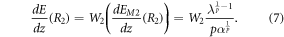
Carbon ions beam lose mainly their energy through Coulomb interactions with electrons, described by the Bethe-Bloch theory. The increased energy loss per unit length as the energy decrease leads to a high energy deposition peak at the end of their range, the BP. The range of a carbon ion beam (R) can be computed using the Bragg-Kleeman rule [10]:

where α and p represent fitting parameters and E0 is the initial beam energy. The range can also be approximated by the position of its BP. The beam deposits energy in the medium between z = 0 and R. At any point, z < R, the remaining energy, E(z), must be enough to travel the distance R − z. In this region, E(z) can be described by:
As Bortfeld showed in 1999 [11], the energy deposited at any point z < R can be computed by the derivative of equation (2):

Assuming that λ represents an infinitesimal distance from the BP position, the energy deposited by a single carbon ion at z = R can be approximated to:

Equations (3) and (4) allow the computation of the energy deposited/intensity at any point of a carbon ion beam crossing a homogeneous medium.
Let one consider an object composed of two materials. The first material is water and represents the surrounding medium. The second material is a cubic block of bone placed inside the surrounding material, as seen in figure 1(a). Therefore, a high gradient interface is created within the surrounding medium. This interface is irradiated with a carbon ion beam parallel to the edge direction. A range detector records the energy of the carbon ion beams at the distal end of the object (figure 1(b)). Due to the heterogeneous medium, range mixing will distort the initial pristine BP signal (expected in a homogeneous medium) into a two BPs signal. The first one corresponds to carbon ions that crossed the densest material (shallow BP at depth R1 after crossing the medium M1) and the other one to carbon ions that crossed the least dense material (deeper BP at depth R2 after crossing the medium M2). Thus, the detector's signal at any point is given by the sum of the deposited energy distributions of carbon ions crossing each interface:

where W1 represents the fraction of carbon ions crossing the densest medium (M1) and W2 the fraction that crosses the least dense medium (M2). Using the prior definitions (i.e. equations (3) and (4)), the intensity of the first BP, located at R1, can be calculated as:

Whereas the intensity of the second BP, located at R2 is defined as:
The fraction of carbon ions that crosses each medium is defined by the distance between the edge and the central position of the irradiation beam. Considering a beam whose lateral distribution is a Gaussian distribution, the distance between the beam and the edge lateral position that would produce the measured fraction of carbon ions crossing each medium can be calculated through the integral of the 2D normal distribution ( ). The relationship is:

where Y is the lateral distance between the beam propagation axis and the edge position. This equation can be solved for Y with the knowledge W1 and W2, which are extracted from equations (6) and (7).
2.2. Edge detection through multiple Bragg peaks: general formalism
The derived formalism can be extended to multiple interfaces and related BPs by measuring all the BP intensities and determining the fraction of carbon ions crossing each interface. Figure 2 represent a detected signal for a phantom producing N BPs. The intensity of the ith BP, located at depth Ri, with ![$i\in [1,N]$](https://content.cld.iop.org/journals/2057-1976/5/6/067002/revision2/bpexab18e6ieqn2.gif) can be calculated by:
can be calculated by:
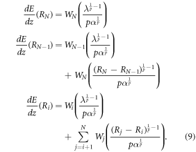
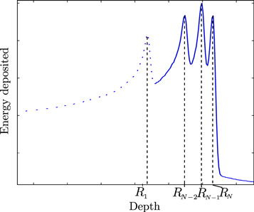
Figure 2. Representation of multiple detected BP. Each BP is positioned at a specific range (RN).
Download figure:
Standard image High-resolution imageFor every BP, the Ri position and the energy deposited at this position ( ) can be measured through the range detector. If λ, p and α are known, the fraction of carbon ions in the last BP (WN) can be calculated. The remaining fractions (
 ,...,Wi) are then iteratively calculated from the second to last
  BPs, up to the i − th BPs (equation (9)).
The final step of the method is to identify the edge of interested and which BPs correspond to carbon ion paths below and above the edge. To do so, prior-knowledge of the edge whereabouts is required. This information can be obtained through the planning CT which will provide an approximation of the edge position. Then, by scanning the assumed edge position with two irradiations beams at two different perpendicular distances (Y) from the edge, the exact edge position can be measured using the technique presented in figure 3. In this example, four BPs were detected in the exit detector. Thus, the incident pencil beam crossed three high-gradient edges parallel to the beam propagation axis. When moving the beam towards the edge of the tumour, W4 decreased, while W3, W2, W1 increased. By assessing the variation of the carbon ions fractions, one can determine the distance to the tumor edge Y, computed using equation (8).

Figure 3. Representation of the Gaussian-shaped lateral distribution of the beam, placed at a edge of high-gradient. In the left figure, the beam is placed at a distance Y from the edge. The same beam crosses materials of different WET, leading to four BP being detected. The fraction of carbon ions crossing each material is given by W1, W2, W3 and W4. By using a second irradiation position, parallel to the previous one, as represented in the right panel, the fraction of carbon ions below the edge (left side of the edge) increases as represented by the bold arrows. Inversely, the fraction of carbon ions above the edge (W4) decreases.
Download figure:
Standard image High-resolution image2.3. Calibrating the irradiation beam parameters
The parameters α, p and λ of equation (7) depend on the detector system and the beam accelerator and transportation system. Thereby, a prior calibration is required. To retrieve them, two carbon ion beams with different energies were propagated through a homogeneous water medium into the range detector. By applying the fit from equation (1), α and p were obtained. λ was calculated using equation (4) with the intensity of the measured BP for a known dose deposition. MC simulations with two beam energies, 300 MeV/u and 400 MeV/u, were considered to simulate such scenario and fit α, p and λ.
2.4. Validation of the model and application in a lung tumor case
In order to assess and validate the derived model, two parametric phantoms with a single high-gradient edge were considered. The first parametric phantom was a water tank with a cubic bone insert of 2 cm thickness (CB2–50% CaCO3 [12]) in the center of the water tank (figure 1). In the second phantom, the cubic insert was replaced by a semi-cylindrical bone insert (radius = 2cm) to produce range dilution effects. Both phantoms were irradiated with carbon ion pencil beams with three different lateral spreads with full width at half maximum (FWHM) of = 4, 8 and 10 mm respectively. To investigate the precision achievable as a function of the distance for each FWHM, the irradiation beam was placed at different lateral distances from the edge (Δy = [−3, −2, −1, 0, 1, 2, 3] mm).
To present a scenario closer to the complexity of a human body, a CT dataset of a patient with a lung tumor from the The Cancer Imaging Archive [13] was used. From the CT, a high-gradient edge was identified between the tumor and the lung tissue. Two directions were selected (figure 5(a)) to crosses the edge. For each direction, five parallel irradiation beams (FWHM = 4mm and spaced 1 mm apart from each other), were propagated through the patient, covering the domain y = [−2, 2] mm around the chosen high-gradient edge.
For all simulations, a water tank (10 × 10 × 20 cm3) was placed at the exit of each phantom in order to simulate a range detector. The energy deposited in the water tank was measured every 0.4 mm along the beam propagation axis. The generated signal was analyzed and the intensities and ranges of all the BPs were measured for each considered lateral distance. The simulations were performed using the Geant4 Monte Carlo simulation code (v4.9.6.p02) [14]. Standard processes include energy loss and straggling, Multiple Coulomb Scattering using the model from [15] and elastic/inelastic ion interactions from dedicated packages of ion interactions provided in Geant4 [16]. The irradiation beam consisted of 105 carbon ions, with an initial energy normally distribution with a mean of 400 MeV/u and an energy spread of 0.4 MeV/u.
3. Results
In order to apply the derived model, the calibration parameters λ, α and p were first determined as explained in section 2.3. Two irradiation beams with two different energy (300 MeV/u and 400 MeV/u both with FWHM = 4 mm) were propagated through a water tank and their ranges measured. By applying the fit from equation (1), p = 1.63 and α = 0.016 were obtained. The parameter λ was determined using equation (4) and by measuring the BP intensity. The calculated value was λ = 0.023.
3.1. Parametric phantoms
This section presents the results for the first two phantoms, i.e. the cubic and the semi-cylindrical inserts. Figure 4 shows the absolute difference between the Y distance found by the algorithm and the known lateral distance, as a function of the later. Figure 4(a) shows the results for the cubic insert while figure 4(b) for the semi-cylindrical insert.
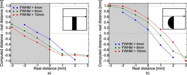
Figure 4. The dots are the absolute computed errors between the computed distance (Y) and the real distance between the beam propagation and the edge. The gray shaded area represents the most dense medium, i.e. below the edge. Three lateral beam sizes were used (FWHM = [4, 8, 10] mm). Figure (a) results were obtained for the phantom with the cube insert (depicted in the left of this figure). Figure b) results were obtained for the semi-cylindrical insert (depicted on the right of this figure).
Download figure:
Standard image High-resolution imageThe BPs intensities and consequently the number of carbons ions that led to each BP dropped greatly when the edge was positioned farther from the beam propagation axis. For a distance to the edge superior to the half of the FWHM of the beam ±1 mm, no multiple BPs were detected. Hence, in order to guarantee a reasonable signal/noise ratio and that multiple BP were detected a Y of FWHM/2 mm was set as the maximal distance from the propagation beam axis that could be detected.
3.2. Lung tumor case
Figure 5(a) shows a representation of two beam directions considered, as explained earlier. Figure 5(b) shows the obtained results for the beam direction Beam1, while figure 6 shows the results obtained for Beam2. Figure 6(a) displays the signal detected on the range detector for a single beam direction.
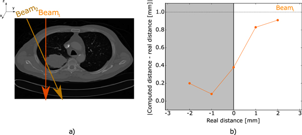
Figure 5. Lung tumor patient case. Figure (a) shows the lung tumor and the two considered beam directions (Beam1, Beam2). Figure (b) shows the results obtained for the beam direction Beam1. It depicts the absolute errors between the computed and the real distances from the beam propagation axis and the edge.
Download figure:
Standard image High-resolution image
Figure 6. Lung tumor patient case. Figure (a) shows the range detector response for all the beams considered for direction Beam2. The light gray area represents the tumor. Figure (b) shows the results obtained for the beam direction Beam2. It depicts the absolute errors between the computed and the real distances from the beam propagation axis and the edge.
Download figure:
Standard image High-resolution image
In order to determine which BPs belonged to the most/least dense medium, the change in the carbon fractions, Wi, was calculated (section 2.2). The results showed a maximal error of 1 mm. A total dose of 23.63 μGy was delivered to retrieve the edge position below a millimiter precision, no matter the direction.
4. Discussion
A theoretical model was derived to calculate the lateral distance between a high-gradient edge and the central position of a pencil beam. The model assumes that multiple BPs are detected after a carbon ion beam crosses a high-gradient edge parallel to the its propagation axis. By measuring the intensity of each BP, the proposed method determines the fraction of carbon ions crossing each medium (equation (7) and equation (9)). These fractions of carbon ions are related to the perpendicular distance between the edge and the propagation axis of the incident beam-Y through the normal distribution (equation (8)).
The proposed method was first tested using two simple phantoms with bony inserts in a water medium; a cubic insert and a semi-cylindrical insert (figure 4). The cubic insert represented a simple scenario, while the semi-cylindrical insert introduced range dilution effects to the measured signal. A smaller mean error was obtained for the cubic phantom with respect to the semi-cylindrical one. This result showed that the range dilution effects caused by the semi-cylindrical shape is a limiting factor of the method. However, range dilution is a smaller issue in carbon imaging since the particles have a more linear trajectory [17].
The impact of the pencil beam FWHM was also studied for the cubic and semi-cylindrical phantoms. Without much surprise, a smaller FWHM led to a higher precision in both phantoms (mean values considering the interval [−2,2] mm: 0.42 ± 0.32 mm for the cubic insert and 0.65 ± 0.28 mm for the semi-cylindrical). In a more complex phantom, such as the lung case, a larger beam lateral size leads to a higher probability of detecting multiple edges parallel to the beam's propagation axis directly increasing the range degradation/dilution effects and leading to multiple BPs.
A lung cancer case was used to reproduce a complex scenario close to the clinical reality. Figure 5(b) and figure 6(b) show the results obtained for the two considered beam directions. The presence of multiple BP required scanning the pencil beam across the edge to measure its position. This was done in order to identify the fraction of carbons crossing the tumor. By measuring the changes in the calculated fractions, the BPs corresponded to carbon ions crossing the tumor were identified (figure 6(a) light gray area.) and the edge position inferred. The error increased as a function of the pencil beam distance to the edge, since the fraction of carbon ions crossing the edge decreased. Even with the complication introduced by a real case, the mean error for the beam direction Beam1 was 0.48 ± 0.33 mm and for the beam direction Beam2, 0.44 ± 0.25. This is due to the fact that the sharp gradient between the tumour and the lung tissue dominates largely over the effect of other interfaces.
The main advantage of the proposed method is that it determined the position of the high-gradient edge accurately (<1 mm) for all investigated scenarios at a very minimal dose cost (24 μGy) and a minimal time.
4.1. Clinical applicability and limitations
This study showed a theoretical approach to confirm and detect the position of high-gradient edges. The detection of two BPs in the measured signal is limited by three factors, the detector quenching and its depth spatial resolution, and the minimum difference between two BP. To minimize the effect of the later a threshold of 3 mm was chosen as a conservative minimum difference between two BPs to be separable. Although BP identification is affected by the detector range resolution, Rinaldi et al [18] have shown a potential resolution of 0.8mm, which is below the imposed limit (3 mm). Nonetheless, these effects might affect the decomposition method and the detector response should be considered in future studies. In addition, respiratory motion effects were also not considered. In a real clinical scenario this effect should be tackled by combining the proposed method with gating strategies. Furthermore, the results obtained in this study may be limited by the two following underlying assumption: (1) the tail of secondary particles in the deposited energy distribution can be neglected and (2) carbon ions can be assumed to travel linearly through the patient. The second assumption has been investigated in Collins-Fekete et al [17]. These limitations and their impacts will be the subject of a subsequent experimental work. Future work could also consider the applicability of this method in imaging reconstruction as means to increase spatial resolution.
5. Conclusion
The irradiation of mediums with different tissue properties, e.g. density, with a high energetic carbon ion beam may lead to the detection of multiple BPs in a range detector. Each BP contains information about the structures that were crossed. In this study, a formalism based on the theoretical definition of a Gaussian beam and the energy deposition curve of carbon ions was derived. The proposed formalism yields the lateral distance between edges and the incident beam propagation axis. The results showed that it is possible to decompose the detected signal and determine the fraction of carbon ions which led to each BP. The method provided information about the position of the edge with a theoretical uncertainty under 1 mm. Potentially, this method could be applied prior to the treatment leading to adaptive treatment with the plan modified from the information returned by this algorithm. This may directly lead to a decrease in the OAR dose. The obtained results did not consider fully the clinical complexity and the technical limitations imposed by an experimental setup. Future work should include testing the proposed methods with other structures where many high-gradient edges are present.
Acknowledgments
This work has been funded by the grant SFRH/BD/85749/2012 from Fundação para a Ciência e a Tecnologia (FCT).