

Abstract
A single human oesophageal adenocarcinoma cell (OE33) has been imaged using aperture infrared scanning near-field optical microscopy (IR-SNOM) in transmission and reflection and also by Fourier-transform infrared (FTIR) microspectroscopy in transmission only. This work presents the first images obtained in both transmission and reflection of the same specimen using the aperture IR-SNOM technique. The results have been used to compare the two SNOM modes and also the two techniques, which have complementary capabilities. The SNOM technique necessitates a very stable source and a careful choice of wavelengths, since it is too slow to yield images at the thousands of wavelengths obtained with FTIR. However the SNOM technique is not diffraction limited and with careful fabrication of tips can yield images with high spatial resolution. There is no significant correlation between the SNOM images obtained in transmission and reflection and the correlations between images obtained at different wavelengths vary with the different imaging modes. These results are attributed to the strong dependence of the evanescent wave on both the wavelength and the distance between the tip and the source of the signal within the sample. While both transmission and reflection SNOM images show some correlation with topography this is not a dominant effect. These results indicate that with suitable calibration a combination of reflection and transmission aperture IR-SNOM measurements has the potential to reveal information on the depth distribution of the chemical structure of a specimen.
Export citation and abstract BibTeX RIS

Original content from this work may be used under the terms of the Creative Commons Attribution 3.0 licence. Any further distribution of this work must maintain attribution to the author(s) and the title of the work, journal citation and DOI.
1. Introduction
There is a need to develop improved techniques for discriminating between benign and malignant tissue excised from patients suspected of developing a variety of cancers. Vibrational imaging techniques, notably Raman spectroscopy and Fourier-transform infrared (FTIR) imaging techniques have considerable potential in this field and have seen significant development and application (Gardner 2016). However both techniques have limited spatial resolution even with the latest optics (Hughes et al 2015): FTIR is limited by diffraction (Pilling and Gardner 2016) and while, in principle, Raman techniques can yield images with submicron scale spatial resolution, this requires high intensity incident beams that can damage the specimen (Amrania et al 2016).
Recently a number of near-field techniques have been developed to overcome the limited spatial resolution of FTIR and Raman spectroscopy. These include scanning near-field optical microscopy (SNOM), which uses an IR-transmitting fiber with an aperture (Smith et al 2013, Halliwell et al 2016) and a family of techniques based on the use of a sharp metal tip to collect the near-field signal; tip-enhanced Raman spectroscopy (Hayazawa et al 2000), scattering scanning near-field optical microscopy (Knoll and Keilmann 1999, Kazantsev and Ryssel 2013, Yoxall et al 2013) and near-field photothermal spectroscopy using a synchrotron (Dazzi et al 2005, Donaldson et al 2016). Each of these near-field techniques has strengths and weaknesses that need to be evaluated before they can provide insight into the development of cancer. This work reports an assessment of one near-field technique, aperture IR-SNOM. Reflection aperture IR-SNOM has previously been used in studies of a variety of systems. Generosi et al (2006) combined IR-SNOM with x-ray reflectivity measurements in studies of solid supported lipid membranes and showed that the SNOM images were not affected by topological artefacts. Cricenti et al (2011) applied the technique to the study of diamond and boron nitride and by tuning the IR source to a DNA absorption signal were able to locate the nucleus of an HaCaT keratinocyte cell. They were also able to determine the location of GluR2 subunits on the surface of neurons by combining IR-SNOM with a fluorophore. This work 'demonstrated the technique can distinguish topological features from lateral variations of the optical properties of the sample'.
We have recently developed transmission IR-SNOM and in the work reported here the results are combined with reflection IR-SNOM in the first application of these techniques to the study of cancer. To the best of our knowledge this is the first study to report images obtained on the same sample using both modes of IR-SNOM. This work also shows FTIR images of the same cell and is the first study to compare the results of IR-SNOM images with FTIR images on biological samples. These two studies are of equal significance and this paper establishes the first links between the three types of images as a precursor to the publication of more detailed studies of cancerous cells and tissue.
2. Experimental details
The SNOM experiments were carried out on the SNOM apparatus, which is installed on the end station (Smith et al 2013) established on the infrared free-electron laser (IR-FEL) of the Accelerators and Lasers In Combined Experiments (ALICE) accelerator. ALICE is an energy recovery accelerator located at the STFC Daresbury Laboratory (Thompson et al 2012). The wavelength of light from the FEL was selected by changing the gap between the magnets in the undulator and, at the beam energy employed, could be varied continuously from about ∼1818 to ∼1136 cm−1 (5.5–8.8 μm). The wavelength of the light was monitored and kept constant using a feedback system. The FEL was operated at a range of powers and the FWHM bandwidth of the IR-FEL light was dependent upon a number of parameters and typically varied from about 23 at 1667 cm−1 (0.09–6.0 μm) to 20 at 1250 cm−1 (0.13–8.0 μm). Recent upgrades (Thompson et al 2015) to ALICE have resulted in improved stability and reduction in long-term drift, with the short-term stability down to 1% when running under optimum conditions. The IR-FEL operates at a macro-pulse repetition rate of 10 Hz, which limits, and determines, the rate of data collection. The IR-light from the FEL was transported to the experimental area through an evacuated beamline and exited the beamline through a KBr window.
The general principle of operation for the SNOM used in these experiments has been described previously (Cricenti et al 2002, 2011). Figure 1 shows a schematic of the IR-SNOM layout used in this work. In brief, higher orders of light from the FEL were filtered out and then the light was attenuated using a set of polarizers. A CaF2 beam-splitter was used to divide the IR-light so that approximately 80% went to the SNOM and 20% was used as a reference signal (Io). The Io signal was monitored with a Gentec-EO UM9B-BL-D0 pyroelectric power meter, which provided a measure of the relative intensity of each macro-pulse. The SNOM images shown in this study were obtained using reflection and transmission mode; reflection has been the standard mode of operation for IR-SNOM. As far as we are aware this is the first use of the IR-SNOM technique in transmission and reflection studies of the same specimen. The SNOM imaging tip was a specially prepared IR-transmitting chalcogenide fiber of core diameter 6 μm sharpened by etching and gold-coated (Unger et al 1998) to create an aperture of ∼0.1 μm in diameter through which the light was collected. The sample was then rastered under the tip, keeping the tip-to-sample distance constant via a feedback mechanism. In reflection mode, the light was focused onto the sample at a grazing incidence angle of approximately 15°. In transmission mode, the FEL beam was perpendicular to the plane of the slide and focused through the CaF2 slide onto the sample. In both cases, the apertured fiber collected the signal in the near-field region above the specimen. The IR-light transmitted through the fiber was detected using a liquid nitrogen cooled mercury–cadmium–telluride (MCT) detector. The SNOM was incorporated into an inverted optical microscope, which was used to locate the specific areas of interest on the sample and to position them within the SNOM scan area. The SNOM instrument used in this study is capable of obtaining images of dimensions ranging from <1 μm up to ∼500 μm and thus enables the study of a wide range of areas and length scales. The lateral resolution of the SNOM images reported in this paper was determined to be ∼0.1 μm, by using the accepted technique of measuring the distance over which a SNOM signal changes from 20% to 80% of the intensity across the sharpest edge of a feature in a small area. The diameter of the aperture of the SNOM fiber is taken to be approximately the same as the measured lateral resolution.
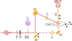
Figure 1. Schematic of the aperture IR-SNOM set-up. The sample was mounted onto a CaF2 slide, which was rastered in the horizontal plane. The chalcogenide fiber (C) moved in the vertical dimension. The SNOM signal was detected using an MCT detector. Shown are the mirrors (M), lenses (L), beam splitter (BS), polarizer (P), filters (F) and the reference detector (Io). The light path for reflection mode is shown by the solid line; the dashed line shows the transmission path. A mirror can be inserted or removed to select the mode.
Download figure:
Standard image High-resolution imageVarious pre-processing techniques were applied to the IR-SNOM images to reduce noise and correct for nonlinearity of the piezoelectric drives before proceeding to image analysis. The first step was to normalize the IR-SNOM signal by dividing it by the Io signal to compensate for fluctuations in the FEL power. It should be noted that the two light paths, to the SNOM and to the Io detector, are not the same and hence the normalization is not ideal. The second step was to correct for the nonlinear response of the piezoelectric drives of the x–y stage of the SNOM. The nonlinearity was first characterized by scanning a grid of known dimensions facilitating the derivation of an algorithmic correction, which was applied to both the topographical and normalized IR-SNOM images. Finally multiple IR-SNOM images were co-registered to take account of small offsets that occur between scans. By comparing the topography of each scan it is possible to overlay, align and then crop all images to a common area, which for the case of most of the images shown in this study was 58 μm × 75 μm. Other common image processing techniques, such as median filtering, were used when appropriate to reduce noise levels without compromising image quality.
Experiments were conducted on a single isolated cell chosen from a culture of OE33 human Caucasian oesophageal adenocarcinoma cells obtained from HPA Culture Collections (Sigma, Dorset, UK) (Rockett et al 1997). Cells were cultured at 37 °C in a 5% CO2 atmosphere in Roswell Park Memorial Institute (RPMI 1640) growth media (Sigma) supplemented with 2 mM glutamine (Sigma), 10% v/v foetal bovine serum (FBS) (Invitrogen, Paisley, UK) and 1% v/v penicillin/streptomycin (Sigma) until they reached 70%–80% confluence. The culture medium was replenished at two-day intervals. CaF2 discs (20 mm diameter × 2 mm thick, Crystran Ltd, Poole, UK) were sterilized using ethanol and rinsed with ultra-pure water and left to air-dry overnight. The discs were irradiated with UV for 30 min to ensure sterility. The sterile discs were then placed in each well of a tissue culture twelve-well plate (Corning, New York, USA). The cells (2 × 10⁴ ml−1) were seeded on each disc and incubated in a 5% CO2 incubator at 37 °C for two-days. After two-days the media was removed and the cells were fixed with a 4% v/v paraformaldehyde (PFA) (Sigma) solution and stored in 1x phosphate buffered saline solution at 4 °C until required. Prior to imaging the CaF2 slide containing the fixed OE33 cells was rinsed at least three times with Millipore ultra-pure water (18 MΩ cm). The rinsed slide was then removed from the well plate, the back surface wiped with ultra-pure water to ensure complete removal of any phosphate residue and then left to dry in the slide holder for a minimum of 90 min.
The cell chosen for imaging was one of medium size, similar in appearance to others of its size and well isolated from other cells and debris. Images of the cell were first obtained with the IR-SNOM operating in transmission mode and then in reflection mode. In each mode images were collected at a single wavelength; topography, SNOM and Io signals were collected simultaneously. The SNOM images show the relative amount of light that was collected by the fiber tip at each pixel. Images of 110 × 110 pixels with a pixel size of 1 μm were collected in 42 min. In both the reflection and transmission SNOM experiments the Io signal intensity was recorded to monitor the (macro) pulse-to-pulse variation of the IR intensity of the FEL beam. Due to time constraints imposed by using accelerator-based facilities it was not possible to image more than one cell of this type. At least 2–4 IR-SNOM images were obtained for each of the conditions to confirm reproducibility.
The culture of OE33 cells was then stored under ambient conditions for seven months after which the same cell was located and FTIR studies of the cell were carried out in transmission with a Varian Cary 670-FTIR spectrometer in conjunction with a Varian Cary 620-FTIR imaging microscope produced by Varian (now Agilent Technologies, Santa Clara CA, USA) with a 128 × 128 pixel MCT focal plane array. For low spatial resolution images, the sample was widely illuminated, ∼1 mm2, and imaged with a field of view of ∼700 × 700 μm giving an image pixel size of ∼5.5 μm. In the high spatial resolution images the optics are changed such that the field of view of the same FPA detector is ∼140 × 140 μm giving an image pixel size of ∼1.1 μm. FTIR images were acquired with a spectral range from 990 to 3800 cm−1 with a spectral resolution of 2 cm−1, co-adding 256 scans. The spatial resolution of the FTIR images is limited to near the diffraction limit.
Infrared spectra were initially pre-processed using a principal component analysis based noise reduction algorithm. Substantial improvements in signal-to-noise were observed by retaining 10 principal components without the loss of biologically significant information. Spectra were then quality checked to remove those not attributable to the cell, or to a high degree of scattering. The quality check utilized a threshold based on the height of the Amide I band with spectra having absorbance between 0.03 and 1.00 being retained. Finally infrared spectra were corrected for resonant Mie scattering with the RMieS-ESMC algorithm using 80 iterations and a matrigel reference spectrum (Marten and Stark 1991, Kohler et al 2008, Bassan et al 2009, 2010). The images were obtained using the high magnification optics consisting of a 0.62 NA objective giving a field of view of 140 μm × 140 μm and a pixel size of 1.1 μm though the images are of course still diffraction limited. The cell was subsequently imaged by a Bruker Innova atomic force microscope (AFM) operated in contact mode, with standard silicon nitride cantilevers and with a spatial resolution of 0.07 μm.
3. Results
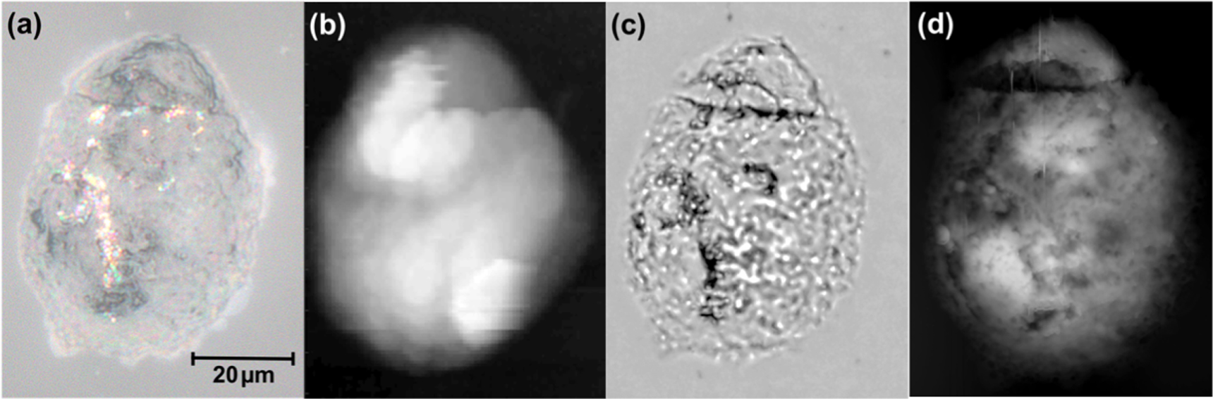
A standard optical microscope image of the cell, taken with a magnification of 400 × (figure 2(a)), shows the cell to be 50 μm × 68 μm in size. Figure 2(b) shows a topographical image obtained with the SNOM fiber tip. A composite depth-of-field image, formed by superposing a sequence of five optical images obtained at different focal planes, reveals subcellular structures (figure 2(c)). The AFM image is shown in figure 2(d). The optical images (figures 2(a) and (c)) were taken approximately 2.5 months after the SNOM images. The high resolution AFM image (figure 2(d)) was acquired at about the same time as the FTIR images, which was about 7 months after the SNOM images. It is difficult to make a direct comparison between the SNOM and AFM images of the topography of the cell, figures 2(b) and (d), since these were obtained with very different spatial resolutions, 2 μm and 0.07 μm respectively. However such a comparison suggests that the topography of the cell has changed slightly during the period between the SNOM and FTIR experiments. Previous experiments with both the IR-SNOM and FTIR techniques have shown that fixed cells are chemically stable over much longer periods (de Stasio et al 1992, Cricenti et al 1996). However in view of the topographic changes the results of the two experiments are evaluated independently.
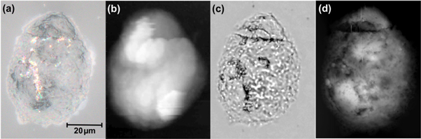
Figure 2. Images of OE33 cell in (a) optical microscope (400×), (b) shear-force SNOM topography, (c) depth-of-field composite microscope and (d) high resolution AFM. The scale-bar in (a) applies to all the images.
Download figure:
Standard image High-resolution imageFigures 3(a) and (b) show respectively the images taken with the SNOM in reflection and transmission at a number of IR wavelengths. It should be noted that the output of the FEL varies significantly over the wavelength range of the images shown in figure 3 and the signal-to-noise level is significantly worse for the image obtained at 1751 cm−1 in reflection than for the other images. Figure 3(c) shows the raw images of the cell obtained with the FTIR in transmission at the corresponding wavelengths and figure 3(d) shows the FTIR images after principal component analysis based noise reduction and a correction for Mie scattering using the RMieS-ESMC algorithm (Marten and Stark 1991, Kohler et al 2008, Bassan et al 2009, 2010).
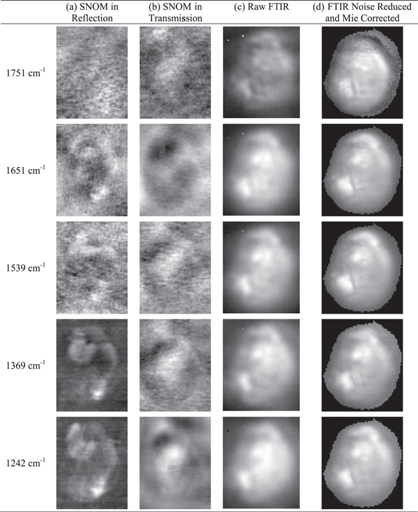
Figure 3. Comparison of SNOM and FTIR images of OE33 cell. (a) SNOM in reflection, (b) SNOM in transmission, (c) raw FTIR images and (d) FTIR images after noise reduction and Mie scattering correction. The SNOM images are 58 μm × 75 μm while the FTIR images are 66 μm × 75 μm. The images have been normalized between 0 (black) and 1 (white).
Download figure:
Standard image High-resolution imageA detailed comparison of the SNOM and FTIR images can be seen in figure 4 which shows the contour plots of the topography and the SNOM images obtained in reflection and transmission at 1242 cm−1 together with the FTIR images of the raw data and the noise reduced and Mie corrected data at the same wavelength.
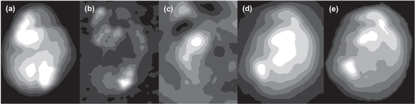
Figure 4. Contour plots showing (a) topography from SNOM reflection, (b) SNOM in reflection at 1242 cm−1, (c) SNOM in transmission at 1242 cm−1, (d) raw FTIR at 1242 cm−1 and (e) noise reduced and Mie scattering corrected FTIR at 1242 cm−1.
Download figure:
Standard image High-resolution image4. Discussion
The strength of the FTIR technique is that images can be obtained over several thousand wavelengths in a reasonably short period of time. Algorithmic techniques such as principal component analysis have been applied to these large data sets and have been shown to yield important information characterizing both cells and tissue (Bassan et al 2012). Although FTIR spectra are influenced by Mie scattering from sub-cellular features, such as the cell nucleus, mitochondria and other organelles, there exist well established techniques for correcting for these effects (Marten and Stark 1991, Kohler et al 2008, Bassan et al 2009, 2010). In this case the Mie scattering correction produced the changes in the intensity distribution of the images shown in figure 3(c) to those of figure 3(d).
In accounting for the differences in the FTIR and SNOM images of figures 3 and 4 it is necessary to consider a number of factors. Firstly the FTIR images are obtained in transmission, at high spectral resolution (2 cm−1) and with a spatial resolution limited by diffraction. The SNOM images are obtained at high spatial resolution but limited spectral resolution (∼20 cm−1). Also, as stated in the previous section, although the cells are fixed and hence no significant chemical variations are expected over this time scale (de Stasio et al 1992, Cricenti et al 1996) comparisons must be made with care. Here, the line profiles of SNOM and FTIR images are compared (figures 5(a) and (b), respectively) for the purpose of highlighting the differing spatial resolutions of the two techniques. These two line profiles are taken 5 μm apart in each image and at roughly corresponding locations within each image. While the line profiles in figure 5(a) vary significantly over short distances, those of figure 5(b) vary only slightly, probably as a consequence of being limited by diffraction.
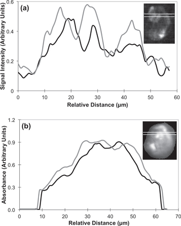
Figure 5. Line profiles through OE33 cell at 1242 cm−1. (a) Line profiles through the SNOM image in reflection mode and (b) line profiles through the noise reduced and Mie corrected FTIR image. The inserts show the locations of the line profiles. The black line profiles are taken from the upper line and the gray line profiles are taken from the lower line through the small insert images.
Download figure:
Standard image High-resolution imageWhile near-field techniques yield images with high spatial resolution, time constraints mean that such images can only be obtained at a limited number of wavelengths. Consequently the choice of wavelengths is an important issue in experiments with SNOM techniques. It is clear from FTIR and Raman techniques that the fingerprint region between 500 and 1500 cm−1 includes key wavelengths that correspond to the main chemical constituents of cells and tissue that are expected to respond to changes induced by disease. Considerable insight into an appropriate choice of spectral biomarkers can be obtained from FTIR studies of proteins, nucleic acids and other biological molecules and there is an extensive literature on the results of such studies (Susi and Byler 1986, Maiti et al 2004, Movasaghi et al 2008, Bellisola and Sorio 2012). It is clear from these studies that the secondary structures of proteins are revealed by the amide bands. In general, each of these bands includes contributions from α-helices, β-sheets and random coils but there is general agreement (Susi and Byler 1986, Maiti et al 2004, Movasaghi et al 2008) that the main peak of the broad Amide I at ∼1650 cm−1 predominately reflects the α-helix structure of proteins and somewhat weaker evidence for associating a peak at ∼1540 cm−1 with the β-sheet structure of proteins. Similarly studies of nucleic acids and lipids indicate that 1242 cm−1  and 1751 cm−1 (C = O lipid ester) are, respectively, a reasonable choice of wavelengths to reflect the contributions of these components of the cell (Movasaghi et al 2008, Bellisola and Sorio 2012). These considerations explain the choice of wavelengths for the images shown in figure 3, though these wavelengths should not be considered too precisely since the IR-FEL had a wide bandwidth of ∼20 cm−1. The wavelength of 1369 cm−1 was chosen as a neutral control since it is not dominated by a single chemical moiety although there is a contribution from the CH3 deformation band of lipids.
In figure 4 neither of the SNOM IR images correlates strongly with the topography and a superficial observation of the reflection and transmission images indicate significant anti-correlation. To quantify the degree of correlation of these images a correlation coefficient was calculated for each pair of images. The correlation coefficient for any two images is a sum over all the pixels in the region of interest (the cell) of the products of the pixel values in the two images, offset from the mean value and normalized by the variance in each image. The correlation coefficient is unity for perfect correlation, zero for no correlation, and minus unity for perfect anti-correlation.
The correlation coefficients of the topography-to-reflection, topography-to-transmission and reflection-to-transmission combinations of the SNOM images shown in figure 4 are 0.43, 0.31 and 0.01 respectively indicating there is a degree of correlation of the IR images with the topography. Figure 6 shows a detailed comparison of the correlation between the SNOM reflection and transmission images obtained at each of the five wavelengths in the form of a color-coded image across the cell with green indicating spatial regions of high correlation and red regions of low correlation together with the corresponding correlation coefficient. The SNOM topographic images obtained in the reflection and transmission experiments are included in this comparison, which reveals a very strong correlation between the two measurements of the topography with a correlation coefficient of 0.97. This result indicates that there was negligible damage to the cell resulting from the scanning by the tip. The correlation coefficients shown in figure 6 demonstrate that there is very little correlation between the reflection and transmission images obtained at each wavelength suggesting that the thickness of the cell (∼2 μm) is responsible for these differences. This result is discussed later.

Figure 6. Correlation plots and coefficients for SNOM in reflection versus SNOM in transmission. The key shows the color-coding used for each of the correlation plots comparing two images. The green diagonal covers pixel values that are similar in image 1 (horizontal axis) and image 2 (vertical axis). The red regions cover pixel values that are significantly different between the two images.
Download figure:
Standard image High-resolution image
Table 1(a) shows the correlation coefficients for all combinations of image pairs for the SNOM images obtained in reflection and table 1(b) the corresponding results for the SNOM images obtained in transmission. Assuming the five wavelengths yield the contributions from the chemical composition of the cell identified above the results of table 1(a) indicate that the SNOM reflection measurements show that the contribution attributed to DNA (1242 cm−1) correlates quite strongly, 0.75, with the image obtained at the control wavelength (1369 cm−1), moderately, 0.39, with the image attributed to β-sheets (1539 cm−1) and poorly, 0.10, with that attributed to α-helices (1651 cm−1). There is a significant correlation, 0.52, between the images attributed to α-helices and β-sheets which is to be expected since both are components of the secondary structure of proteins. The image obtained from the lipids (1751 cm−1) shows very little correlation with any of the other constituents when measured in reflection, a result which should not be taken too seriously given the poor signal-to-noise of the lipid image. A comparison of tables 1(a) and (b) reveals some subtle differences between the image correlations obtained with the SNOM in reflection and in transmission. The DNA image and the image obtained at the control wavelength show a similar degree of correlation in transmission as in reflection, ∼0.75. The correlation between the DNA image and the images attributed to both the β-sheet and α-helices, 0.74 and 0.20 respectively, approximately doubles in transmission compared to the corresponding results obtained in reflection. There is a similar though slightly smaller correlation, 0.39, between the images obtained for the α-helices and β-sheets in transmission compared with the results obtained in reflection, 0.52. The contribution from the lipids correlates quite strongly with contributions from DNA, β-sheets and the control wavelength, 0.66, 0.70 and 0.74 respectively when measured in transmission but only weakly with the contribution from the α-helices, 0.11. The poor signal-to-noise of the lipid image measured in reflection obviates a meaningful comparison of the correlations involving the lipid images obtained in reflection and transmission. These detailed differences between the SNOM images obtained in reflection and transmission are considered later.
Table 1. (a) Pixel correlation coefficients for SNOM in reflection. (b) Pixel correlation coefficients for SNOM in transmission.
| 1751 cm−1 | 1651 cm−1 | 1539 cm−1 | 1369 cm−1 | 1242 cm−1 | Topography | |
|---|---|---|---|---|---|---|
| a | ||||||
| 1751 cm−1 | 1.00 | 0.08 | 0.03 | −0.01 | −0.05 | −0.03 |
| 1651 cm−1 | 0.08 | 1.00 | 0.52 | 0.24 | 0.10 | −0.40 |
| 1539 cm−1 | 0.03 | 0.52 | 1.00 | 0.57 | 0.39 | −0.08 |
| 1369 cm−1 | −0.01 | 0.24 | 0.57 | 1.00 | 0.75 | 0.38 |
| 1242 cm−1 | −0.05 | 0.10 | 0.39 | 0.75 | 1.00 | 0.43 |
| Topography | −0.03 | −0.40 | −0.08 | 0.38 | 0.43 | 1.00 |
| b | ||||||
| 1751 cm−1 | 1.00 | 0.11 | 0.70 | 0.74 | 0.66 | 0.25 |
| 1651 cm−1 | 0.11 | 1.00 | 0.39 | 0.22 | 0.20 | −0.43 |
| 1539 cm−1 | 0.70 | 0.39 | 1.00 | 0.70 | 0.74 | 0.08 |
| 1369 cm−1 | 0.74 | 0.22 | 0.70 | 1.00 | 0.74 | 0.26 |
| 1242 cm−1 | 0.66 | 0.20 | 0.74 | 0.74 | 1.00 | 0.31 |
| Topography | 0.25 | −0.43 | 0.08 | 0.26 | 0.31 | 1.00 |
Tables 2(a) and (b) show respectively the results of the pairwise correlations obtained for the raw and the noise reduced and Mie corrected FTIR images of figure 3. The tables include correlations between the FTIR images and the topography of the cell obtained by the AFM. The first thing to note is that all the raw FTIR images show strong correlations with the topography, 0.85–0.95. These correlations are reduced slightly following the correction for Mie scattering but this reduction arises mainly from an apparent shrinking of the cell outline, an artefact resulting from the thresholding that is applied when the Mie correction is applied. The strong correlation of the FTIR images with the topography obtained by AFM is consistent with the results that the FTIR images obtained at different wavelengths also show strong correlations with each other that in some cases are slightly reduced by the Mie scattering correction. The conclusion from the results of these correlation studies is that the FTIR results are more strongly influenced by the topography, and hence the thickness of the cell, than by variations in its chemical composition. While it is possible, in principle, to compensate for the effect of the thickness, i.e. topography, of the cell using vector normalization, when this was applied the resultant images showed no significant contrast. We believe this is a consequence of the chemical signature of the images being a small fraction of the contribution from the topography. Thus the images can be thought of as a strong topographic signal being modulated by a smaller chemical signal. The fact that the signal is dominated by topography, rather than chemistry, does not preclude quantitative data analysis because the latter deals with a large data set of spectral profiles obtained over several thousand wavelengths at each pixel, thus allowing the chemical information to be extracted.
Table 2. (a) Pixel correlation coefficients for raw FTIR images. (b) Pixel correlation coefficients for noise reduced and Mie corrected FTIR images.
| 1751 cm−1 | 1651 cm−1 | 1539 cm−1 | 1369 cm−1 | 1242 cm−1 | Topography | |
|---|---|---|---|---|---|---|
| a | ||||||
| 1751 cm−1 | 1.00 | 0.75 | 0.90 | 0.89 | 0.81 | 0.86 |
| 1651 cm−1 | 0.75 | 1.00 | 0.78 | 0.85 | 0.90 | 0.84 |
| 1539 cm−1 | 0.90 | 0.78 | 1.00 | 0.97 | 0.88 | 0.93 |
| 1369 cm−1 | 0.89 | 0.85 | 0.97 | 1.00 | 0.94 | 0.94 |
| 1242 cm−1 | 0.81 | 0.90 | 0.88 | 0.94 | 1.00 | 0.94 |
| Topography | 0.86 | 0.84 | 0.93 | 0.94 | 0.94 | 1.00 |
| b | ||||||
| 1751 cm−1 | 1.00 | 0.96 | 0.94 | 0.94 | 0.94 | 0.93 |
| 1651 cm−1 | 0.96 | 1.00 | 0.97 | 0.97 | 0.97 | 0.97 |
| 1539 cm−1 | 0.94 | 0.97 | 1.00 | 1.00 | 1.00 | 1.00 |
| 1369 cm−1 | 0.94 | 0.97 | 1.00 | 1.00 | 1.00 | 1.00 |
| 1242 cm−1 | 0.94 | 0.97 | 1.00 | 1.00 | 1.00 | 1.00 |
| Topography | 0.93 | 0.97 | 1.00 | 1.00 | 1.00 | 1.00 |
The results of tables 1(a) and (b) demonstrate that unlike the correlations deduced for the FTIR images the cell topography does not dominate the SNOM images. This is brought out very clearly in the images of the OE33 cell shown in figures 4(a)–(c), which show respectively the topography and the images obtained at 1242 cm−1 in reflection and transmission. These images are expected to show the DNA content of the cell. Clearly the strength of the DNA signal is influenced more by the inhomogeneous distribution of the DNA in the cell than by the topography and this distribution is characterized with high spatial resolution in two dimensions. However as demonstrated by figure 4 and the correlation results of figure 6 for all the chosen wavelengths the images obtained in reflection are quite different from the images obtained in transmission. Since the distribution of chemical moieties in the cell does not change between reflection and transmission, these observations raise the issue of the extent to which SNOM experiments can reveal the depth distribution of the chemical structure of the cell. The thickness of the OE33 cell as measured by AFM is ∼2.3 μm and the distance between the SNOM tip and the specimen surface is ∼0.02 μm. Over the wavelength range the whole of the specimen is in the near-field region. However, the evanescent waves that are collected by the SNOM aperture fall off rapidly in intensity with distance, d, from the tip. A simple model based on the fields around a point-like oscillating dipole (Cricenti and Perfetti 2007) suggests that the intensity of the signal from the SNOM will vary as k2/d4 where k is the wavenumber of the radiation generated by the dipole, and d is the distance between the dipole and the SNOM aperture. Although this simple model does not describe the full complexity of how the signal at the detector is generated by the fields in the near-field region (i.e. by the evanescent waves) around the source, it should give a rough indication of the dependence of the signal on wavenumber and distance. The optical image, figure 2(c), indicates that there is a significant variation in the composition of the cell with depth and this coupled with the dependence of the evanescent wave on depth is the most likely explanation of the difference in the two dimensional distribution of DNA observed in the reflection and transmission images in figures 4(b) and (c). This can be seen from a consideration of the k2/d4 term, which indicates that over this wavenumber range the intensity observed from a molecule reduces by almost two orders of magnitude as the molecule is moved 1 μm deeper into the specimen. The dependence of the evanescent wave on wavenumber can also account for the differences in the correlation coefficients for all combinations of image pairs for the SNOM images obtained in reflection and transmission (tables 1(a) and (b)). This is because, over this wavenumber range, the intensity of signals obtained at different wavenumbers from a molecule at a fixed depth can vary by between 30% and 50%. It may be possible to calibrate the SNOM signal in order to obtain depth information by studying specimens of known variation in composition similar to the technique used to calibrate the Mie scattering contributions to FTIR spectra (Bassan et al 2009). The benefits of such a calibration can be judged from the three-dimensional images of cells obtained in recent work combining infrared and optical techniques (Zhang et al 2016). In the absence of such a calibration it is clear that while the SNOM can give accurate information on the lateral spatial variation of DNA the sensitivity of the evanescent wave to wavelength makes it difficult to quantify the variation of the chemical composition with depth.
5. Conclusions
This comparison of images taken of the same cell at the same wavelengths with the aperture IR-SNOM technique and the more established FTIR microspectroscopy technique has confirmed the expected strengths and weaknesses of the two techniques. The SNOM technique is too slow to yield images at the thousands of wavelengths obtained with FTIR, which necessitates a careful choice of wavelengths, though this choice cannot be too precise given the 20 cm−1 bandwidth of the IR-FEL employed in this study. However the SNOM technique is not diffraction limited and with careful fabrication of tips can yield images with high spatial resolution. The current instrument is capable of imaging an area of 100 μm × 100 μm with a pixel size of 1 μm in an hour and in previous work has yielded spatial resolution of ∼0.1 μm over smaller areas (Smith et al 2013). The stability of the source is a crucial determinant of the signal-to-noise obtained with the SNOM and the results presented in this work are crucially dependent on the stability achieved in operating the IR-FEL.
This work presents the first images obtained in both transmission and reflection of the same specimen using the aperture IR-SNOM technique. There is no significant correlation between the SNOM images obtained in transmission and reflection and the correlations between images obtained at different wavelengths vary with the different imaging modes. These results are attributed to the strong dependence of the evanescent wave on both the wavelength and the distance between the tip and source of the signal within the sample. While both transmission and reflection SNOM images show some correlation with topography this is not a dominant effect. These results indicate that with suitable calibration the aperture IR-SNOM technique has the potential to reveal information on the depth distribution of the chemical structure of a specimen.
It is suggested that the complementary capabilities of the aperture IR-SNOM and FTIR microspectroscopy techniques have considerable potential when used in combination to yield insight into the chemical structure of biological systems.
Acknowledgments
This work was supported by the UK Engineering and Physical Sciences Research Council (UK EPSRC: Grant No. EP/K023349/1). JI and TC acknowledge support from EPSRC studentships. PG acknowledges the Williamson Trust for funds for the FTIR Imaging system. The authors acknowledge and express thanks to the following: All ASTeC staff who were key commissioners running ALICE and Daresbury staff who provided endless support; Prof. George King, University of Manchester for his help, support and for acting as a second commissioner and Dr Chris Edmonds, Cockcroft Institute for acting as a second commissioner.