

Abstract
Two ferritic stainless steel (FSS) specimens, denoted as loading axis along the rolling direction(LR) and the transverse direction(LT) respectively, were produced to elucidate the mechanical anisotropyof409L FSS at grain scale. This approach was realized by the combination of in situ tensile test and field emission scanning electron microscopy (SEM) with electron backscattering diffraction (EBSD) at room temperature. Microstructure evolution, grain orientation rotation, and crystallographic slip were investigated in the tensile test. During tensile deformation, the tensile axis of LR specimens rotated towards the 〈101〉 direction, which is the stable end orientation of body-centered cubic (BCC) metals. However, the rotation of tensile axis towards 〈101〉 was restrained in LT specimens due to the operation of less favorable slip systems. {110}〈111〉 was the most favorable slip system in both specimens. The mechanical anisotropy in grain scale is due to different slip behaviors of LR and LT specimens.

Original content from this work may be used under the terms of the Creative Commons Attribution 4.0 licence. Any further distribution of this work must maintain attribution to the author(s) and the title of the work, journal citation and DOI.
1. Introduction
Ferritic stainless steel (FSS) has been applied in various industries [1–3]. It is considered as an interesting substitute for austenitic stainless steel because of its high thermal conductivity, small linear expansion, better resistance to chloride stress-corrosion cracking and low cost. However, FSS still suffers from several problems [4], one of which is ridging. When pulling or deep drawing, FSS shows undesirable surface corrugation along the rolling direction. In the past few decades, the causes of ridging have drawn much attention. It is generally believed that coarse banded structure of colonies [5], known as grain colonies, is responsible for ridging. Different grain colonies and matrix are likely to show different plastic anisotropies [4–6], leading to ridging. In almost every process of FSS manufacturing, such as casting [5, 7, 8], hot rolling [9, 10] and cold rolling [4, 8], the correlation between grain colonies and ridging has been observed. Furthermore, ridging-free FSS was produced through recrystallization of lath marten site [11], in which there were no grain colonies.
However, there were almost no successful attempts to complete suppression of ridging in traditionally manufactured FSS. Wright's observation showed that ridging was the most severe when pulling along the rolling direction and less severe when the angle with the rolling direction increases. According to Lee et al [12], the sample deformed at 90° to RD showed the most severe ridging. These conflicts indicate that the influence of mechanical anisotropy introduced by grain colonies on FSS remains unclear. In addition, in terms of FSS mechanical anisotropy, most studies focus on texture [12, 13] and corresponding modeling [14]. There are few experimental studies on grain scale, such as orientation rotation, crystallographic slip, and the correlation between them. In particular, almost no literatures have experimentally studied the tensile deformation and related mechanisms in FSS, such as the correlation between grain orientation rotation and active slip systems, which are essential to understand the fundamental mechanism of FSS deformation.
In recent years, with the development of EBSD and tensile stages within SEM, orientation information and corresponding microstructure evolution during tensile deformation can be obtained. Jiang et al [15] investigated the effect of grain orientation rotation on plastic deformation of single crystal super alloy. Zhang et al [16] studied the microstructure evolution of duplex stainless steel with in situ EBSD. Kawano et al [17] studied an in situ EBSD of the orientation and slip systems in commercial pure titanium crystal. Liu et al [18] applied in situ SEM analysis to investigate the slip and deformation mechanism of ferrite in low carbon steel. Nonetheless, detailed grain scale studies on FSS anisotropic grain orientation rotation and crystallographic slip are still lacking.
In this work, in situ SEM uniaxial tensile tests with EBSD of two FSS specimens, denoted as LR (loading axis along the rolling direction) and LT (loading axis along the transverse direction), were pulled along the rolling direction (RD) and the transverse direction (TD). Microstructure evolution and grain orientation rotation in both specimens during the tensile test were recorded and compared. Slip trace analysis were conducted to determine the active slip systems of both specimens.
2. Materials and methods
Hot-rolled and annealed 409 L ferritic stainless steel sheet with a thickness of 5.0 mm was applied in this study. Its chemical composition is shown in table 1. After removing the oxide layer by pickling in 200 ml HCl+800 ml H2O and grinding with 400# water proof abrasive paper, the sheet was cold-rolled from 4.8 mm to 0.5 mm, and the thickness was reduced by nearly 90%. Then the sheet was recrystallized and annealed in a vacuum furnace(3.0 × 10⁻³ Pa at 880 °C for 5 min).Two tension specimens, denoted as LR (loading axis along the rolling direction) and LT (loading axis along the transverse direction), were obtained from the sheet by spark erosion wire cutting. The specimen dimensions and in situ experiment setup are shown in figure 1. Two specimens were mechanically polished and then electrochemically polished in 25% perchloric acid solution at 0°C for 20 s. After final polishing, the thickness of specimens was 0.25 mm.
Table 1. Chemical composition of 409 L ferritic stainless steel (wt%).
| C | N | Si | Mn | P | S | Ti | Nb | Ni | Cr | Fe |
|---|---|---|---|---|---|---|---|---|---|---|
| 0.0083 | 0.0096 | 0.29 | 0.33 | 0.0029 | 0.002 | 0.221 | 0.012 | 0.07 | 11.50 | Bal. |

Figure 1. Experiment setup for in situ tensile deformation for EBSD analysis: (a) dimensions of the tensile specimen (in millimeter) and two specimens with loading direction along RD and TD, denoted as LR (loading axis along the rolling direction) and LT (loading axis along the transverse direction), respectively; (b) tensile stage with a tensile specimen (tilted at 70°about the horizontal direction) used for in situ EBSD analysis.
Download figure:
Standard image High-resolution imageAs shown in figure 1(b), a SEM tensile stage (Gatan Inc.) was implemented to perform in situ uniaxial tensile deformation at room temperature. The strain level ( ) can be evaluated according to equation (1):

where L represents the distance of parallel length of the specimen(the distance from A to B in figure1(a)), ad L0 is the initial distance from A to B, with 12 mm.
Three successive strain levels of 3.6%, 5.4% and 7.2% were achieved for LR and LT specimens. The crosshead speed in the tensile stage was maintained at 0.1 mm min−1, corresponding to an initial strain rate of about 10−5s−1.
EBSD data was obtained using an Apollo 300 SEM (ObducatCamScan Ltd.) equipped with Aztec software package (Oxford Instruments) at an acceleration voltage of 20 kV. The step size was 1μm for all EBSD mapping. Before and after deformation of LR (figure 2) and LT (figure 3) specimens, a region of approximately 200 × 200μm2 near the center of the tensile specimen was mapped using EBSD. At each successive tensile deformation interval, the secondary electron image was captured in the same area for slip trace analysis.

Figure 2. Orientation maps at different strains of LR specimens, bar = 50 μm, (a) 0%, (b) 3.6%, (c) 5.4% and (d) 7.2%.
Download figure:
Standard image High-resolution image
Figure 3. Orientation maps at different strains of LT specimen, bar = 50 μm, (a) 0%, (b) 3.6%, (c) 5.4%, and (d) 7.2%.
Download figure:
Standard image High-resolution imageAztec and ATEX software were applied for EBSD data processing. For LR and LT specimens, more than 93% of the pixels were indexed in the initial state. As the deformation accumulated, the index rate dropped below 90%, especially near the grain boundaries. After noise reduction, the index rate was more than 99%. The grain tolerance angle adopted a 5° threshold, excluding grains less than or equal to 2 pixels.
3. Results and discussion
3.1. Microstructure evolution
Figures 2 and 3 illustrate the orientation maps of LR and LT specimens at different strain intervals during the in situ tensile tests. The inverse pole figure (IPF) maps show the grain orientations with respect to the normal direction (ND). Figures 2(a) and 3(a) show the recrystallized microstructures of 409 L FSS after cold rolling and annealing, and the grain colonies with 〈111〉∥ND and 〈011〉∥ND are observed. Before tension deformation, each grain had a uniform orientation, and the average grain size was 52.4 μm and 46.8 μm for LR and LT specimens, respectively. At 3.6% strain shown in figures 2(b) and 3(b), the studied regions are slightly elongated. Accordingly, only a small amount of IPF color in the grains deviates from the initial orientations, indicating that there is heterogeneous deformation in these regions. With the strain increases to 5.4% and 7.2%, IPF color varies remarkably inside the grain, indicating that crystal orientation rotations occurs gradually. In addition, twins were not observed in either LR or LT specimens, because abrupt color changes and parallel boundaries within the grains were not spotted in both orientation maps.
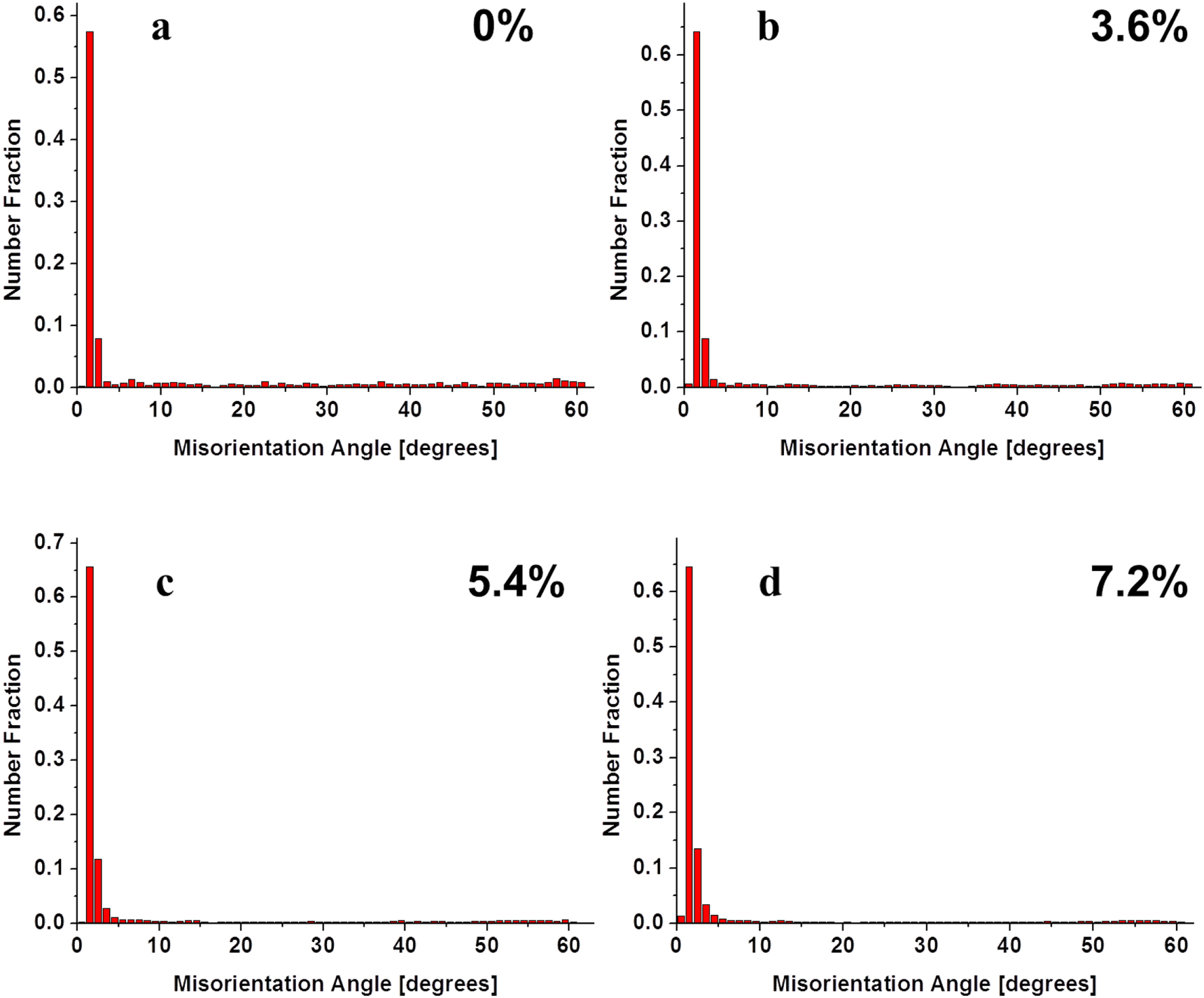
Figure 4 shows the orientation angle distributions of LR specimens at different strains. In the unstrained state, 51.9% of the boundaries are low-angle boundaries (LABs), that is, boundaries with misorientations of less than 15°, and the remaining 48.1% of the boundaries are high-angle boundaries (HABs), where the misorientation is greater than 15°. Most grain boundaries are LABs, which broadly indicates the existence of grain colonies. At 3.6% strain, the fraction of LABs boundaries increases to 64.0%. Moreover, as the strain reaches 5.4%, the fraction of LABs increases to 78.5%, and this number rises to 82.7% at 7.2% strain.

Figure 4. Misorientation angle distributions of LR specimens at different strains, (a) 0%, (b) 3.6%, (c) 5.4%, and (d) 7.2%.
Download figure:
Standard image High-resolution imageFigure 5 shows the misorientation angle distributions of LT specimens at different strains. In the unstrained state, 74.3% of the boundaries are LABs. At 3.6% strain, 81.4% of the boundaries are LABs, which rises to 86.3% and 88.8% at 5.4% strain and 7.2% strain, respectively. The significant increase of LABs in both specimens is due to geometrically necessary dislocations (GNDs). Generally, plastic deformation of body- centered cubic (BCC) metalsisrealized by dislocation motion. The dislocation structure is usually divided into two components: statistically stored dislocations (SSDs), and geometrically necessary dislocations (GNDs). The latter contributes to curvatures and fragmentation of crystallite lattice [19]. When the metals are imposed with strain, GNDs rise and correspondingly further forms sub grain boundaries [17], resulting in an increase in LABs. In addition, no twinning was observed in LR and LT specimens at room temperature. The formation of deformed twinning during the in situ tensile test will significantly increase the faction of misorientation angle at 60°, because the orientation relationship of the twin boundary of BCC material is 〈111〉 60°. According to figures 4 and 5, only the rising of LABs was observed, indicating that slip is the only deformation mechanism for 409 L FSS.

Figure 5. Misorientation angle distributions of LT specimen at different strains, (a) 0%, (b) 3.6%, (c) 5.4%, and (d) 7.2%.
Download figure:
Standard image High-resolution image3.2. Evolution of crystallographic texture
To investigate the evolution of crystallographic texture of LR and LT specimens during uniaxial tensile deformation, the IPF contoured maps with respect to normal direction (ND) and loading direction (rolling direction (RD) for LR specimens and transverse direction (TD) for LT specimens) are shown in figures 6 and 7.

Figure 6. Inverse pole figures contoured maps of LR specimens at different strains, (a) 0%, (b) 3.6%, (c) 5.4%, and (d) 7.2%. Z represents ND relative to crystal-based coordinate, and X represents RD relative to crystal-based coordinate.
Download figure:
Standard image High-resolution image
Figure 7. Inverse pole figures contoured maps of LT specimens at different strains, (a) 0%, (b) 3.6%, (c) 5.4%, and (d) 7.2%. Z represents ND relative to crystal-based coordinate, and Y represents TD relative to crystal-based coordinate.
Download figure:
Standard image High-resolution imageFor LR specimens, the initial micro-texture is shown in figure 6(a). In ND, the most preferred orientation lies around 〈112〉 and 〈111〉, which is 3.28 times the random. In RD, the strongest orientation lies near 〈123〉, with 2.89 times the random. As the strain increases from 0 to 7.2%, the orientation distribution is relatively stable in ND. Moreover, at 7.2% strain, the most preferred orientation remains 〈112〉, and the intensity is about3.12 times the random. On the contrary, a clear orientation rotation is observed in RD. With the strain increases from 0 to 7.2%, the most preferred orientation rotates from the initial orientation towards 〈101〉, and the intensity rises to 4.56 times the random. This result is in consistent with the previous works of BCC metals: low carbon micro-alloyed steel [20] and coarse-grained tantalum [21].
For LT specimens, the initial micro-texture is shown in figure 7(a). In ND, the most preferred orientation is about 〈111〉, and the intensity is 3.87 times the random. In TD, the preferred orientation is between 〈122〉 and 〈133〉, and the intensity is 2.69 times the random. As the strain increases from 0 to 7.2%, the most preferred orientation remains 〈111〉, and the orientation density rises from 3.87 to 5.60 times the random in ND. However, in TD, the most preferred orientation rotates from the initial position to 〈101〉 at 3.6% strain, and then stops and spreads with the preferred orientation intensity dropping from 2.69 to 2.49 times the random.
Obviously, the loading directions can distinguish the orientation rotation behavior of 409 L FSS, that is, the orientation of tensile axis determines the rotation behavior in the tensile test. It is believed that 〈101〉 orientation is a stable end orientation during uniaxial tension of BCC metals [22]. A comparison of the rotational behavior of tensile axis between two low-carbon steel [20] specimens indicates that different slip activities may result in different rotation behaviors of the two specimens. It is thus deduced that the active slip systems may determine the orientation rotation behaviors of BCC metals. When loading along the rolling direction, the grains are relatively easy to rotate towards the stable end orientation 〈110〉. For LT specimens, when loading along the transverse direction, the rotation towards 〈110〉 was somehow restrained, and different slip behaviors may result in the unusual rotation behaviors. It is thus necessary to investigate the active slip systems in two FSS specimens.
3.3. Slip trace analysis
To further investigate the active slip systems of 409 L FSS, a slip trace analysis is performed. Using the local grain orientations obtained from EBSD, possible active slip systems can be calculated. The comparison between the calculated active slip lines and observed slip lines will further reveal the active slip system. This analysis had been utilized in a variety of metals and alloys, such as pure magnesium [23], titanium alloy [24] and duplex stainless [25]. Due to the complexity of the slip planes in BCC metals [26], it is assumed that there are 48 possible slip systems in FSS, including 12 {110}〈111〉 slip systems, 12 {112}〈111〉 slip systems, and 24{123}〈111〉 slip systems. The methodology to determine the active slip systems contains the following steps: (1) determine the Euler angles (φ1, ϕ, φ2) according to the grain orientations, where the slip lines were observed in the secondary electron images; (2) calculate the slip line angles of all possible slip systems with the previous Euler angles; (3) select the slip system that matched the observed slip line. If there are several slip lines that match the observed slip lines, we assume that the slip system corresponding to the highest Schmid factor is activated.
In order to minimize the orientation index errors, a slip trace analysis is conducted on LR and LT specimens at the first strain interval of 3.6%. There are 91 and 108 grains in LR and LT specimens, respectively. The grains are marked with the same number generated by the 'show Grains ID' tool in the ATEX software. As shown in figures 8 and 9, the grains with clear straight slip lines are selected for slip trace analysis, and this method cannot apply wavy and fuzzy slip lines. In addition, black and colored lines are used to represent the observed and calculated slip lines, respectively. The {110}〈111〉 slip systems are highlighted in red lines; {112}〈111〉 slip systems are highlighted in green lines, and {123}〈111〉 slip systems are highlighted in blue lines. A 5°angle between the observed and calculated slip lines is used as the threshold.

Figure 8. Slip traces in LR specimens at 3.6% strain, (a) IPF map and grain number, (b), (c) and (d) secondary electron images with overlaid slip lines, black lines represent the observed slip lines and colored lines represent the calculated slip lines. {110}〈111〉 slip systems were highlighted in red lines, {112}〈111〉 slip systems were highlighted in green lines, and {123}〈111〉 slip systems were highlighted in blue lines.
Download figure:
Standard image High-resolution image
Figure 9. Slip traces of LT specimens at 3.6% strain, (a) IPF map and grain number, (b), (c) and (d) secondary electron images with overlaid slip traces, black lines represent the observed slip lines and colored lines represent the calculated slip lines. {110}〈111〉 slip systems are highlighted in red lines; {112}〈111〉 slip systems are highlighted in green lines, and {123}〈111〉 slip systems are highlighted in blue lines.
Download figure:
Standard image High-resolution imageFigure 8 shows the slip traces of LR specimens at 3.6% strain. Either the grain boundaries or the slip lines could be clearly visualized in the secondary electron images as a result of plastic deformation. The slip lines are relatively straight and mainly spotted near the grain boundaries, that is, strain concentration occurred around the grain boundaries. In several grains, more than a slip system are identified in one grain, such as grain G58 (figure 8(c)), where the slip lines matching {110}〈111〉 and {112}〈111〉 slip systems are observed. It is worth noting that different slip systems observed in a grain are located in different regions of the grain, which indicates that the crystal rotation behavior in a grain is inhomogeneous. With further strain, the misorientation between different regions increases, leading the formation of sub grain boundaries. As shown in table 2, 32 slip lines in 25 grains are identified in LR specimens, where the average disparity angle between the observed and calculated slip lines is1.4°. In these 32 slip lines, 11 match the {110}〈111〉 slip system; 8 match the {112}〈111〉 slip system, and 13 match the {123}〈111〉 slip system. In addition, the average Schmid factor (absolute value) is 0.42, 0.37, and 0.33 corresponding to the observed {110}〈111〉, {112}〈111〉, and {123}〈111〉 slip systems, respectively. It fits well with the fact that the planes with the largest interplanar spacing are {110}, followed by {112}, and then {123}. However, it is worth noting that the Schmid factors of grains G80 and G52 are 0.03 and −0.05, respectively. The extreme low Schmid factor (〈±0.1) is highlighted with bold type in tables 2 and 3.
Table 2. Grain number, observed and calculated slip line angles, slip systems and corresponding Schmid factors of LR specimens at 3.6% strain for the regions denoted in figure 8. Extreme low Schmid factors are in bold.
| Grain | Observed slip line angle/° | Calculated slip line angle/° | Slip system | Schmid factor |
|---|---|---|---|---|
| G20 | 136.8 | 136.4 | (10)[11] | 0.49 |
| G58 | 67.1 | 67.5 | (10)[11] | −0.37 |
| G55 | 132.4 | 130.7 | (10)[11] | 0.49 |
| G75 | 34.6 | 38.3 | (01)[11] | −0.42 |
| G71 | 129.5 | 130.1 | (101)[11] | −0.41 |
| G70 | 47.9 | 45.5 | (01)[11] | −0.47 |
| G76 | 44.6 | 42.7 | (01)[11] | −0.47 |
| G44 | 13.3 | 13.8 | (110)[11] | −0.17 |
| G84 | 45.3 | 43.6 | (01)[11] | −0.49 |
| G73 | 59.6 | 61.9 | (10)[11] | 0.41 |
| G64 | 141.2 | 144.8 | (10)[11] | 0.44 |
| G58 | 138.5 | 139.8 | (11)[111] | −0.33 |
| G34 | 36.3 | 37.3 | (12)[11] | −0.37 |
| G20 | 144.8 | 145.3 | (21)[11] | 0.38 |
| G56 | 135.8 | 135.9 | (12)[11] | −0.41 |
| G72 | 135.5 | 137.7 | (12)[11] | 0.43 |
| G66 | 42.8 | 43.3 | (121)[11] | −0.38 |
| G87 | 140.8 | 140.2 | (12)[11] | −0.38 |
| G18 | 147.1 | 147.3 | (211)[11] | −0.24 |
| G55 | 142.5 | 141.3 | (32)[11] | −0.46 |
| G80 | 44.7 | 44.3 | (21)[111] | 0.03 |
| G30 | 46.1 | 43.4 | (13)[11] | 0.45 |
| G37 | 30.5 | 28.0 | (13)[11] | −0.34 |
| G43 | 50.9 | 48.7 | (32)[11] | 0.27 |
| G87 | 145.4 | 146.8 | (13)[11] | −0.42 |
| G64 | 41.6 | 41.8 | (13)[11] | −0.49 |
| G63 | 139.7 | 137.3 | (13)[11] | −0.37 |
| G52 | 144.3 | 144.2 | (12)[111] | − 0.05 |
| G47 | 143.4 | 145.2 | (13)[11] | −0.41 |
| G18 | 40.5 | 40.0 | (13)[11] | −0.45 |
| G44 | 138.8 | 135.6 | (23)[11] | −0.40 |
| G89 | 48.6 | 51.8 | (312)[11] | −0.21 |


Table 3. Grain number, observed and calculated slip line angles, slip systems and corresponding Schmid factors of LT specimens at 3.6% strain for the regions denoted in figure 9. Extreme low Schmid factors are in bold.
| Grain | Observed slip line angle/° | Calculated slip line angle/° | Slip system | Schmid factor |
|---|---|---|---|---|
| G50 | 135.2 | 136.6 | (110)[11] | −0.37 |
| G41 | 136.1 | 136.6 | (110)[11] | −0.37 |
| G41 | 44.4 | 43.9 | (011)[11] | −0.37 |
| G64 | 135.0 | 137.5 | (011)[11] | 0.34 |
| G69 | 115.9 | 115.8 | (011)[11] | −0.39 |
| G49 | 108.0 | 107.6 | (01)[111] | −0.47 |
| G22 | 141.3 | 144.0 | (011)[11] | 0.27 |
| G31 | 58.8 | 58.9 | (10)[111] | 0.44 |
| G31 | 131.8 | 129.3 | (011)[11] | −0.36 |
| G56 | 24.4 | 26.5 | (01)[11] | −0.26 |
| G45 | 44.5 | 46.3 | (11)[111] | −0.10 |
| G45 | 111.8 | 110.7 | (121)[11] | −0.23 |
| G36 | 50.3 | 52.0 | (112)[11] | −0.19 |
| G14 | 138.5 | 142.2 | (121)[11] | − 0.04 |
| G33 | 51.6 | 52.2 | (21)[11] | −0.36 |
| G32 | 43.4 | 43.9 | (211)[11] | −0.15 |
| G50 | 15.1 | 16.6 | (121)[11] | − 0.03 |
| G4 | 132.2 | 131.0 | (13)[11] | −0.48 |
| G5 | 42.5 | 44.2 | (31)[11] | 0.40 |
| G6 | 112.6 | 115.1 | (23)[11] | −0.39 |
| G42 | 46.7 | 45.6 | (12)[111] | −0.23 |
| G36 | 37.8 | 36.6 | (123)[11] | −0.19 |
| G50 | 20.7 | 20.3 | (12)[111] | −0.24 |
| G65 | 29.5 | 31.2 | (321)[11] | 0.03 |
| G65 | 138.4 | 135.8 | (21)[111] | 0.08 |
| G64 | 40.7 | 42.0 | (213)[11] | 0.25 |
| G68 | 122.0 | 121.5 | (13)[11] | −0.14 |
| G69 | 38.6 | 37.6 | (31)[11] | 0.38 |
| G74 | 132.5 | 130.3 | (312)[11] | −0.17 |
| G19 | 121.5 | 120.7 | (31)[11] | −0.22 |
| G28 | 137.6 | 137.5 | (13)[11] | 0.38 |
| G56 | 39.3 | 39.8 | (13)[11] | −0.33 |
| G11 | 136.4 | 139.4 | (312)[11] | −0.44 |
| G44 | 48.1 | 49.7 | (132)[11] | −0.21 |
| G39 | 140.8 | 139.6 | (21)[111] | 0.04 |
| G13 | 39.7 | 42.4 | (31)[11] | 0.39 |
| G12 | 55.3 | 53.2 | (312)[11] | −0.11 |


For LT specimens shown in figure 9, similar to LR specimens, the straight slip lines and grain boundaries are observed in the secondary electron images. There are 37 slip traces in 27 grains of LR specimens, and the average disparity angle between the observed and calculated slip lines is also 1.4°. Among these slip traces, 10 match {110}〈111〉; 7 match{112}〈111〉 and 20 match {123}〈111〉. The average Schmid factor (absolute value) is 0.36, 0.16 and 0.26 corresponding to the observed {110}〈111〉, {112}〈111〉, and {123}〈111〉 slip systems, respectively. However, there are 4 grains (grain G14, G50, G65 and G39) with low Schmid factors. Unlike monocrystals, the general deformation of BCC polycrystals requires at least five active slip systems, and the strain distribution generated by slip is inhomogeneous. Extreme low Schmid factors in both specimens are the consequence of local strain concentration during tensile deformation.
Despite the inconformity of Schmid's law, the Schmid factor is the most commonly used approach to predict deformation behavior of individual grains in BCC metals [27], because non-Schmid parameters are temperature-dependent and have small effect at room temperature [28]. The average Schmid factor of {110}〈111〉 slip system is higher than that {112}〈111〉 and {123}〈111〉 for LT and LR specimens. The {110}〈111〉 slip systems are more likely to operate in advance for LR or LT specimens. According to the average Schmid factor, the {112}〈111〉 and {123}〈111〉 slip systems are less favorable slip systems. Moreover, the average Schmid factor of LR specimens is higher than that of LT specimens in each slip system, which means that less favorable slip systems are operated while loading along the transverse direction, that is, to adapt to tensile deformation, less favorable slip systems were operated in LT specimens compared to LR specimens. This verifies the assumption that different slip behaviors influence the orientation rotation behaviors of LT specimens. Given the fact that the grains in the two specimens correspond to different Schmid factors, the deformation in each grain may vary, leading to further strain localization.
The calculated Maximum Schmid factor (MSF) distribution of all grains shown in figures 8(a) and 9(a) is shown in figure 10. Assuming that the slip only occurs on a set of planes, such as the {110} planes, the highest Schmid factor in each grain is calculated and the distribution is plotted in the form of a red histogram. For LR specimens in figure 10(a), the maximum Schmid factor in the three slip systems is mainly between 0.4 and 0.5. Moreover, MSF{123}〈111〉 > MSF{110}〈111〉 > MSF{112}〈111〉, that is, {123}〈111〉 is the most favorable slip system, followed by{110}〈111〉then{112}〈111〉. In contrast, the maximum Schmid factor of LT specimens has a wider distribution and MSF {123}〈111〉 > MSF{112}〈111〉 > MSF{110}〈111〉. This result supports the ideal that compared with LR specimens, less favorable slip systems are operated to accommodate the tensile deformation of LT specimens. However, MSF{123}〈111〉 is the largest in LR and LT specimens, indicating that{123}〈111〉 is the most favorable slip system, which is inconsistent with the results of slip trace analysis. That is because the calculation of MSF only takes into account the orientations of grains. In FSS polycrystalline, slip activities are more complex.

Figure 10. Distribution of calculated maximum Schmid factor of (a) LR and (b) LT specimens.
Download figure:
Standard image High-resolution image
4. Conclusion
In this work, in situ EBSD tensile tests were conducted on two 409 L FSS specimens with different loading direction at room temperature. Combined with the evolution of microstructure and grain orientation during tensile deformation and the slip trace analysis, the following conclusion can be drawn:
- 1.The grain colonies were observed in 409 L FSS annealing. The geometrically necessary dislocations (GNDs) were responsible for the significant increase of LABs in LR and LT specimens during the tensile tests. Moreover, no twinning was observed, and the slip was the only deformation mechanism at room temperature.
- 2.The orientation rotation behaviors of grains in LR and LT specimens were different. For LR specimens, the tensile axis rotated towards 〈110〉, which is the stable end orientation of BCC metals. For LT specimens, the rotation of tensile axis towards 〈110〉 was restrained, which was caused by the operation of less favorable slip systems.
- 3.The slip trace analysis indicates that the three slip systems {110}〈111〉, {112}〈111〉 and {123}〈111〉 are operated and {110}〈111〉 is the most favorable slip system of LR and LT specimens.
- 4.The mechanical anisotropy in grain scale is due to different slip behaviors of LR and LT specimens.
Acknowledgments
The authors would like to acknowledge the financial support by Natural Science Foundation of China (Grant No. 51171103).
Data availability statement
The data generated and/or analysed during the current study are not publicly available for legal/ethical reasons but are available from the corresponding author on reasonable request.