Using constrained mixture design method for optimizing the properties of organoclay filled ethylene-octene copolymer nanocomposites

Masoud Tayefi; Mohammad Razavi-Nouri; Alireza Sabet

doi:10.1088/2053-1591/ab61aa

1. Introduction

In conventional one-factor-at-a-time approach, only one variable is altered while the others are kept constant. Therefore, using this method is time consuming and expensive. Moreover, the technique is unable to identify interactions among the factors [1, 2]. Design of Experiment (DoE) methods, which are now extensively applied to analyze the influence of multi factors on the responses, allows us to study a number of factors simultaneously [3, 4]. Experimental designs are classified in three general types, namely; screening method, response surface and mixture design. Screening designs such as factorial design (FD) and fractional factorial design (FFD) are mainly employed to identify the most significant factors affected on a response [5, 6]. It is worth to mention that the traditional experimental design methods, such as FD, assume that all variables can be controlled and operated independently of one another. In a composite material experiment, this could be attained if a researcher is only concerned in varying one or two components engaged [7]. The response surface methods (RSM) such as Box-Behnken design, central composite and mixture designs will initially aid users to study the effects of the factors on each property of a material by carrying out an affordable number of experiments [4, 8–13]. Moreover, the interactions between the factors can be evaluated by the method [14–16]. In addition, the designed experiments could help an experimenter to find the nonlinear relationships between the factors and properties studied [17, 18]. Besides process optimization, RSM methods are capable of producing an approximate continuous surface and contour plots for evaluating the interactions [18–20]. It should also be mentioned that while central composite and Box–Behnken designs are largely carried out when the factors are process variables, mixture design is employed for formulation factors [15]. In mixture design, the sum of all ingredients of a mixture is assumed to be 100% or 1 except when any constant mixture factors are present. The shape of the experimental zone will be a simplex if all mixture factors change from 0 to 100% [21]. In many cases, the preparation of the mixtures in the whole range of proportion values of their components, may not be of any interest or even impossible to be studied. Thus, it could be suitable to establish low and high constraints for a number of components [22]. Where the factors have different limitations, the restricted experimental zone turns into an irregular polyhedron within the simplex [21]. The mixture design method has extensively been employed to study and model the influence of compositions on different properties of a variety of mixtures such as polymers and other materials [15–17, 22–25].

Ethylene-1-octene copolymers (EOCs) are made from the copolymerization of ethylene and 1-octene [26]. The new class of the copolymer is now synthesized by metallocene single site catalysts [27]. EOCs show outstanding physical and mechanical properties such as resistance to solvents, high elongation at break, environmental resistance and dielectric properties. Therefore, they can be used in the form of blends and composites in a variety of applications [28].

The preparation of polymer-based nanocomposites has comprehensively been investigated during the past two decades due to their unique physical and mechanical properties. Among the nanofiller used, polymer/organoclay (OMT) nanocomposites have received widespread attentions because of their attractive behaviors and potential applications in many areas [29, 30].

Cross-linking (curing) is also widely used to improve the thermal and mechanical properties of some polymers, especially elastomers. Peroxides are among the cross-linking agents and have numerous advantages compared to other curatives or curing agents [31].

The main objective of this work is to analyze the significance of EOC, dicumyl peroxide (DCP) and OMT content on different physical and mechanical properties of the EOC-based nanocomposites using a constrained mixture design approach. Five responses of tensile strength, modulus at 100% strain, strain at break, XRD peak intensity and the initial slope of the logarithm of storage modulus (G') versus the logarithm of angular frequency (ω) at the terminal zone were selected for this evaluation. The results were employed to determine the mixture design models for the properties investigated. The contour plots were then applied to understand the effect of each component on individual responses and finally the optimum formulation was proposed.

2. Experimental

2.1. Materials

EOC (LC370) with 38 wt% octene content, density of 0.87 g cm⁻³ and MFI of 3.0 g/10 min (190 °C/2.16 kg) was supplied from LG Chem Ltd (South Korea). Cloisite 15 A (C15A) with the interlayer spacing of 31.5 Å, density of 1.66 g cm⁻³ and cation exchange capacity of 125 meq/100 g was purchased from Southern Clay Products (USA). Dihydrogenated tallow dimethyl ammonium was used as a modifier for C15A. DCP with the purity of 99% was supplied from Concord Chemical Ind. Co. Ltd (Taiwan) and used as a cross-linking agent.

2.2. Sample preparation

In order to remove any traces of moisture, C15A was dried in a vacuum oven at 80˚C for 24 h before being mixed with the other materials. The nanocomposites were prepared using a two-step melt mixing method. All of the mixtures were prepared using a Brabender internal mixer (Germany) equipped with a pair of roller blades. EOC/C15A masterbatch containing 10 wt% OMT was first prepared at 60 rpm and 100 °C for 10 min. The mixture was then diluted with the addition of appropriate amounts of EOC to prepare the nanocomposites containing 1 to 5 wt% C15A. The rotor speed, temperature and mixing time were set to be 60 rpm, 150 °C and 5 min, respectively. The nanocomposites were also dynamically cured using 0.5 and 1 wt% DCP. Reaching the mixing torque to its maximum value was selected as criteria to finish the cross-linking stage and remove the nanocomposites from the mixer. Square plaques with the thickness of 1 mm were then prepared by compression molding of the materials at 150°C and 15 MPa for 5 min using a Toyosiki Mini Test Hydraulic Press (Japan).

2.3. Low angle X-ray diffraction

The X-ray analysis of each sample was carried out using a X'pert PRO MRD X-ray diffractometer (PANalytical, The Netherlands) operated with CuKα radiation (λ = 1.542 Å) at 40 kV and 40 mA. The 2θ angles in the range 0.7°–10° with an exposure time of 2 s and scanning rate of 0.02 °/s was selected to scan the samples.

2.4. Mechanical properties

A Universal Testing Machine (Santam-SMT20, Iran) was employed to determine the tensile properties of the nanocomposites. At least five dumbbell-shaped specimens with 35 × 2 × 1 mm³ dimensions were punched out from the plates for each composition and tested with the cross-head speed of 500 mm min⁻¹. The results obtained were then averaged to find the mean and standard deviation values.

2.5. Rheological properties

A stress controlled rheometer (Anton Parr MCR501, Austria) was used to study the rheological behavior of the samples. Disk-type parallel plates with 25 mm diameter and 1 mm gap were employed to determine the dynamic oscillatory shear responses of the nanocomposites in their linear viscoelastic regions. The values of G' were obtained in the range 0.01–100 rad s⁻¹ of ω at the temperature of 110 °C and strain of 0.5% under a nitrogen atmosphere.

3. Experimental design

According to the mixture design method, the formulations of a series of EOC-based nanocomposites were considered with three components of EOC, DCP and OMT. In this work, the amount of OMT and DCP were selected to be in the range 1–5 wt% and 0–1 wt%, respectively. This is because, the physical and mechanical properties of the nanocomposites were unfavorably decreased or at most remained nearly unchanged beyond the two values mentioned above.

To model the system, the scale of the mixture design should be modified owing to the existence of some constraints for the components selected. A lower-bound pseudo-component was considered for our system to find the fitting model. The lower pseudo-components (X_i values) were determined using the following equations [32];

$\begin{eqnarray}&&{X}_{i}=\displaystyle \frac{{R}_{i}-{L}_{i}}{100-L}\end{eqnarray} \tag{ 1 }$

where i = 1, 2, 3, ..., n and

$\begin{eqnarray*}&&L=\displaystyle \sum _{i=1}^{n}{L}_{i}\end{eqnarray*}$

$\begin{eqnarray*}&&\displaystyle \sum _{i=1}^{n}{X}_{i}=1\end{eqnarray*}$

where R_i is the real value and L_i is the lower bound of each component. In this study n=3; demonstrated as the number of mixture variables in this work (X₁, X₂, and X₃). The range of actual components and corresponded pseudo-components are shown in table 1. Figure 1 shows the schematic layout of the design. As it can be seen, a parallelogram shaped image containing nine design points is constructed due to the applied constraints. For confirmation of the accuracy of the models obtained by experimental design, one additional point located inside of the experimental region was also considered. Design-Expert^® software version 10 was employed to analyze the effects of the components on the properties evaluated in this study. A regression was performed on the experimental data wherein the responses were estimated according to practical correlations between the predicted responses and the components. To fit a model containing the components studied, the least square technique was utilized. It was carried out by the minimization of the residual error measured via the sum of square deviations between the real and predicted responses. This includes the approximations of the regression coefficients, i.e. the coefficients of the models' components and the intercepts. It is worth to mention that, the statistical significance of the computed coefficients of the equations should then be examined. Therefore, three examinations were executed to evaluate (1) the significance of the regression model, (2) the significance of each coefficient of the models and (3) the lack of fit. Moreover, each examination should be carried out to check whether the model could explain the experimental data. This was achieved, in this work, by calculating the various coefficients of determination (R²) in which their values vary in the range 0 to 1. Additionally, the capability of the model was also studied by checking of residuals [4]. The term describes the difference between the predicted and the observed responses. The residuals were checked here using the normal probability plots of the residuals and the plots of the residuals against the responses predicted by the models. The points on the former plots should form a straight line, if the model is satisfactory. Furthermore, the points on the latter plots should not form any specific structure, i.e., no obvious pattern should be detected.

Table 1. Real proportions of the components in the mixture and in pseudo-components.

	Range of each component (wt%)		Pseudo-component value
Mixture components	Low	High	Symbol	Low	High
EOC content	94	99	X₁	0	1
DCP content	0	1	X₂	0	0.2
OMT content	1	5	X₃	0	0.8

**Figure 1.** Layout of the mixture design with its constraints for the three components (the values in the bracket define the pseudo-component of each component at that specific point).
Download figure:
Standard image High-resolution image

A three component mixture design method was adopted to find a correlation between the responses which are the tensile strength, modulus at 100% strain, strain at break, XRD peak intensity and the initial slope of log Gʹ against log ω. The linear, quadratic and special cubic models were employed to achieve the best accurate model to fit the experimental results. The models are as follow;

$\begin{eqnarray}&&{\rm{Y}}={\alpha }_{1}{{\rm{X}}}_{1}+{\alpha }_{2}{{\rm{X}}}_{2}+{\alpha }_{3}{{\rm{X}}}_{3}\end{eqnarray} \tag{ 2 }$

$\begin{eqnarray}&&{\rm{Y}}={\alpha }_{1}{{\rm{X}}}_{1}+{\alpha }_{2}{{\rm{X}}}_{2}+{\alpha }_{3}{{\rm{X}}}_{3}+{\alpha }_{12}{{\rm{X}}}_{1}{{\rm{X}}}_{2}+{\alpha }_{13}{{\rm{X}}}_{1}{{\rm{X}}}_{3}+{\alpha }_{23}{{\rm{X}}}_{2}{{\rm{X}}}_{3}\end{eqnarray} \tag{ 3 }$

$\begin{eqnarray}&&{\rm{Y}}={\alpha }_{1}{{\rm{X}}}_{1}+{\alpha }_{2}{{\rm{X}}}_{2}+{\alpha }_{3}{{\rm{X}}}_{3}+{\alpha }_{12}{{\rm{X}}}_{1}{{\rm{X}}}_{2}+{\alpha }_{13}{{\rm{X}}}_{1}{{\rm{X}}}_{3}+{\alpha }_{23}{{\rm{X}}}_{2}{{\rm{X}}}_{3}+{\alpha }_{123}{{\rm{X}}}_{1}{{\rm{X}}}_{2}{{\rm{X}}}_{3}\end{eqnarray} \tag{ 4 }$

where Y represents the responses (dependent variables) and all the α_i values are the numerical coefficients of the models.

The experimentally determined results are listed in table 2. It is worth to mention that the number of runs required for the analysis was 10 i.e. 9 for the pseudo-component values used in the analysis and 1 for replication of the center point. It should also be noted that the figures related to the X-ray diffraction response and rheological behavior of the materials studied have been reported earlier by the authors [33].

Table 2. The proposed compositions according to the mixture design method and their mechanical properties, XRD peak intensities and rheological values.

	Pseudo-components			Dependent variables
Run	EOC	DCP	OMT	Tensile strength (MPa)	Modulus at 100% strain (MPa)	Strain at break (%)	XRD peak intensity (Counts)	Slope of log G' versus log ω
1	1	0	0	11.27 ± 1.09	2.03 ± 0.05	1846 ± 171	6464	1.33
2	0.9	0.1	0	6.62 ± 0.01	2.53 ± 0.07	807 ± 79	6421	0.40
3	0.8	0.2	0	8.92 ± 0.39	5.19 ± 0.12	193 ± 32	2823	0.23
4	0.6	0	0.4	14.83 ± 0.77	1.97 ± 0.09	2167 ± 134	15002	1.27
5	0.5	0.1	0.4	8.27 ± 0.30	2.66 ± 0.03	817 ± 36	11369	0.37
6^a	0.5	0.1	0.4	8.00 ± 0.33	2.69 ± 0.02	800 ± 30	11485	0.36
7	0.4	0.2	0.4	9.35 ± 0.47	6.23 ± 0.30	182 ± 35	5221	0.22
8	0.2	0	0.8	15.65 ± 0.57	1.92 ± 0.09	2196 ± 88	22594	1.22
9	0.1	0.1	0.8	8.13 ± 0.29	2.91 ± 0.14	808 ± 61	17549	0.32
10	0	0.2	0.8	9.82 ± 0.35	6.21 ± 0.12	176 ± 7	7014	0.19

^aReplication of the center point.

4. Results and discussion

4.1. Analysis of variance for all responses

The analysis of variance (ANOVA) was carried out in order to quantify the effects of selected components and their interactions on the dependent variables. The significance of each term can be determined based on its probability value (P-value). Significant term should have the probability value more than 95% (P-value ≤ 0.05) and the probability of insignificant term will have the value less than 95% (P-value ≥ 0.05) [34, 35]. Therefore, the insignificant terms were omitted here from the final analysis and results.

The ANOVA results for the analysis of tensile strength, modulus at 100% strain, strain at break, XRD peak intensity and the initial slope of log Gʹ against log ω are tabulated in tables 3 to 7, respectively. Table 3 reveals that a special cubic model can be used to fit the tensile strength response. The P-value of the model was calculated to be 0.0007 (probability of >99%) which is in agreement with the fact that the model was highly significant. On the contrary, the P-value of lack of fit (0.3958) indicated that the lack of fit was insignificant and the model fitted the data satisfactorily. The interactions between the components of EOC*DCP, EOC*OMT, DCP*OMT and EOC*DCP*OMT were significant with the P-value of 0.0003 (probability of >99%), 0.0150 (probability of ≈99%), 0.0003 (probability of >99%) and 0.0436 (probability of ≈96%), respectively.

Table 3. Analysis of variance for tensile strength.

Factor	SS^a	Df^b	MS^c	F-value	P-value
Model	80.09	6	13.35	172.11	0.0007
Linear mixture	38.78	2	19.39	250.03	0.0005
EOC*DCP	30.66	1	30.66	395.29	0.0003
EOC*OMT	1.98	1	1.98	25.52	0.0150
DCP*OMT	30.54	1	30.54	393.78	0.0003
EOCDCPOMT	0.88	1	0.88	11.31	0.0436
Residual	0.23	3	0.078
Lack of fit	0.20	2	0.098	2.69	0.3958
Pure error	0.036	1	0.036
Cor total	80.33	9

^aSum of Square: Sum of the squared differences between the average values and the overall mean. ^bDegree of freedom. ^cMean of Square: Sum of squares divided by the degree of freedom. F-value: Test for comparing term variance with residual variance.P-value: Probability of seeing the observed F-value if the null hypothesis is true. Residual: Consists of terms used to estimate the experimental error.Lack of fit: Variation of the data around the fitted model. Pure error: Variation in the response in replicated design points.Cor total: Totals of all information corrected for the mean.

Table 4. Analysis of variance for modulus at 100% strain.

Factor	SS	Df	MS	F-value	P-value
Model	0.14	4	0.035	267.25	< 0.0001
Linear mixture	0.13	2	0.067	511.59	< 0.0001
EOC*DCP	5.213E-003	1	5.213E-003	39.66	0.0015
DCP*OMT	4.287E-003	1	4.287E-003	32.61	0.0023
Residual	6.573E-004	5	1.315E-004
Lack of fit	6.514E-004	4	1.629E-004	27.71	0.1414
Pure error	5.878E-006	1	5.878E-006
Cor total	0.14	9

Table 5. Analysis of variance for strain at break.

Factor	SS	Df	MS	F-value	P-value
Model	1.69	6	0.28	5530.42	< 0.0001
Linear mixture	1.66	2	0.83	16223.25	< 0.0001
EOC*DCP	0.031	1	0.031	615.30	0.0001
EOC*OMT	6.614E-004	1	6.614E-004	12.95	0.0368
DCP*OMT	0.027	1	0.027	524.18	0.0002
EOCDCPOMT	5.449E-004	1	5.449E-004	10.67	0.0469
Residual	1.532E-004	3	5.106E-005
Lack of fit	1.115E-004	2	5.574E-005	1.34	0.5217
Pure error	4.170E-005	1	4.170E-005
Cor total	1.69	9

Table 6. Analysis of variance for XRD peak intensity.

Factor	SS	Df	MS	F-value	P-value
Model	3.489E + 008	4	8.723E + 007	519.03	< 0.0001
Linear mixture	3.050E + 008	2	1.525E + 008	907.53	< 0.0001
EOC*DCP	8.241E + 006	1	8.241E + 006	49.04	0.0009
DCP*OMT	2.834E + 006	1	2.834E + 006	16.86	0.0093
Residual	8.403E + 005	5	1.681E + 005
Lack of fit	8.335E + 005	4	2.084E + 005	30.97	0.1339
Pure error	6728.00	1	6728.00
Cor total	3.497E + 008	9

Table 7. Analysis of variance for the slope of log G' versus log ω.

Factor	SS	Df	MS	F-value	P-value
Model	0.97	4	0.24	1319.10	< 0.0001
Linear mixture	0.91	2	0.46	2474.08	< 0.0001
EOC*DCP	0.060	1	0.060	325.44	< 0.0001
DCP*OMT	0.060	1	0.060	325.05	< 0.0001
Residual	9.231E-004	5	1.846E-004
Lack of fit	8.523E-004	4	2.131E-004	3.01	0.4048
Pure error	7.080E-005	1	7.080E-005
Cor total	0.98	9

Table 4 shows that a quadratic model can be suitable to fit the modulus at 100% strain with the P-value of <0.0001 (probability of >99%). The P-value of lack of fit was found to be 0.1414, revealing its insignificance. The two-component interactions of EOC*DCP and DCP*OMT were significant with the P-value of 0.0015 and 0.0023 (probability of >99%), respectively. However, the P-value of EOC*OMT was more than 0.05 which means that the interaction was not significant. Therefore, the interaction was eliminated from the equation.

In order to fit the strain at break, a special cubic model was recommended according to the data presented in table 5. The analysis of variance for the model showed that the P-value of the model was less than 0.0001 (probability of >99%) and the P-value of lack of fit was 0.5217. Consequently, the model was convincing from statistical point of view without any significant lack of fit in the range of the components examined. The interactions of EOC*DCP, EOC*OMT, DCP*OMT and EOC*DCP*OMT were effective for the determination of the values of the strain at break with the P-value of 0.0001 (probability of >99%), 0.0368 (probability of >96%), 0.0002 (probability of >99%) and 0.0469 (probability of >95%), respectively.

As it can be observed in table 6, a quadratic model with the P-value of <0.0001 (probability of >99%) could be suggested to fit the XRD peak intensity results. It should be noted that the lack of fit was insignificant with the P-value of 0.1339. The interactions of EOC*DCP and DCP*OMT were significant in calculating the XRD peak intensity values with the P-value of 0.0009 (probability of >99%) and 0.0093 (probability =99%), respectively. However, the effect of EOC*OMT was negligible due to its high P-value which was more than 0.05. Therefore, this interaction was omitted from the equation.

The analysis of variance showed that a quadratic model could be used to fit the initial slope of log G' against log ω (see table 7). The P-value of the model was less than 0.0001 (probability of >99%) and that of lack of fit was 0.4048. This was also consistent with the fact that the model was statistically convincing and fitted the results successfully. The two-component interactions of EOC*DCP and DCP*OMT were effective in influencing the initial slope of log G' versus log ω with the P-value of <0.0001 (probability of >99%) for both. However, the P-value of EOC*OMT was higher than 0.05, indicating that the interaction was not effective in evaluating the quantity. Therefore, this two-component interaction was eliminated from the results.

The regression coefficients and their standard errors for all the models are tabulated in table 8. The models are based on the pseudo-component coding.

Table 8. The estimated regression coefficients and their standard errors for the models obtained.

Coefficients and their errors	Tensile strength	(Modulus at 100% strain)^−0.5	Log₁₀ (Strain at break)	XRD peak intensity	Log₁₀ (Initial slope of log G' versus log ω)
α₁	11.35	0.71	3.27	6460	0.13
Standard error	0.27	9.93 × 10^–3	6.85 × 10^–3	355	0.01
α₂	304.45	−4.37	−11.38	−160269	9.02
Standard error	15.27	0.60	0.39	21409	0.71
α₃	14.64	0.72	3.33	27026	0.07
Standard error	0.55	0.01	0.01	462	0.02
α₁₂	−380.68	4.66	12.19	185300	−15.82
Standard error	19.15	0.74	0.49	26462	0.88
α₁₃	9.37		0.17
Standard error	1.85		0.05
α₂₃	−393.07	4.31	11.64	110681	−16.11
Standard error	19.81	0.75	0.51	26953	0.89
α₁₂₃	−49.19		−1.23
Standard error	14.62		0.38

In addition, a brief statistics of the best model for each response is tabulated in table 9. The value of R² can also be used as a criterion in order to evaluate the ability of the models to predict the results. A model can estimate the result more accurately if the value is much closer to 100%. As it can be observed, the R² values obtained from the analysis are 99.71 for tensile strength, 99.53 for modulus at 100% strain, 99.99 for strain at break, 99.76 for XRD peak intensity and 99.91 for initial slope of log G' versus log ω. The high values of R² for all the properties investigated are consistent with the fact that the proposed models are highly capable in predicting the responses in the range studied.

Table 9. The statistics of the best model selected for each response.

Response	Model	R-Squared (%)	Adj. R-Squared (%)	Pred. R-Squared (%)
Tensile strength	Special Cubic	99.71	99.13	93.03
Modulus at 100% strain	Quadratic	99.53	99.16	96.76
Strain at break	Special Cubic	99.99	99.97	99.82
XRD peak intensity	Quadratic	99.76	99.57	98.73
Slope of log Gʹ versus log ω	Quadratic	99.91	99.83	99.40

It is worth to mention that R²–adj. (adjusted determination coefficient) of all responses was also near to 100%. The values also confirmed that the significance of the models were high. The predicted R² (Pred. R-Squared) values were also in good agreement with the adjusted R² (Adj. R-Squared) values.

The appropriate amounts (pseudo-component) of X₁, X₂ and X₃ were substituted in the models in order to compare the experimental data, for each response, with those values calculated from the models. For instance, for sample 4 (0.6, 0, 0.4), the experimental and predicted values were found to be 14.83 and 14.92 MPa for tensile strength, 1.97 and 1.97 MPa for modulus at 100% strain, 2167 and 2152% for strain at break, 15002 and 14686 counts for XRD peak intensity and finally 1.27 and 1.27 for the initial slope of log G' versus log ω, respectively. As another example, sample 10 (0, 0.2, 0.8), it was established that the experimental and predicted values were obtained to be 9.82 and 9.72 MPa for tensile strength, 6.21 and 6.62 MPa for modulus at 100% strain, 176 and 176% for strain at break, 7014 and 7276 counts for XRD peak intensity as well as 0.19 and 0.19 for the initial slope of log G' versus log ω, respectively. The results showed that there was very good agreement between the experimental and predicted data in all cases studied.

The normal probability plots of the studentized residuals for the models are shown in figures 2(a) to (e). These plots can be useful for checking the capability of a model to fit the data set [2, 36]. The points located on the normal probability plots of the residuals should form a straight line if the model is sufficient [37]. All the figures indicate that the residuals form a straight line in agreement that the errors are normally distributed.

**Figure 2.** Normal probability plots of studentized residuals for (a) tensile strength, (b) modulus at 100% strain, (c) strain at break, (d) XRD peak intensity and (e) the slope of log G' versus log ω.
Download figure:
Standard image High-resolution image

Figures 3(a) to (e) illustrate the plots of the residuals versus the predicted responses. All plots showed that the residuals did not form any reasonable pattern. These are consistent with the fact that the models suggested for the responses are quite suitable and there is no reason to be worried about any violation of the independence or constant variance assumption [3].

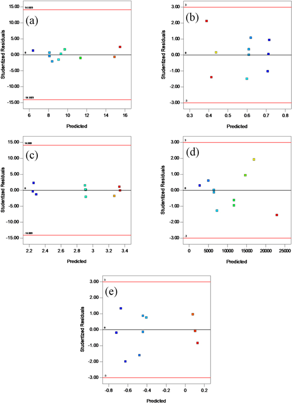
**Figure 3.** Plots of the residuals against predicted responses for (a) tensile strength, (b) modulus at 100% strain, (c) strain at break, (d) XRD peak intensity and (e) the slope of log G' versus log ω.
Download figure:
Standard image High-resolution image

4.2. Contour plots

The influence of combination of the mixture ingredients on the magnitude of responses are depicted in figures 4(a) to (e) in the form of 2D contour plots. The plots have been divided into several sections in which the variations of the colors' of different regions reveal the trend of responses. The sections with darker colors are related to responses with higher magnitudes in comparison with those of brighter colors. Various magnitudes of responses and coordinating points and thus the proportion of components could be evaluated by passing through different regions in contour plots. Figure 4(a) shows that the high tensile strength values (higher than 14 MPa) can be obtained in the region illustrated by red color at the edge of EOC-OMT. The highest values were determined for formulations 4 and 8 with the values of 14.83 and 15.65 MPa, respectively. The former was made of 0.6 EOC, 0 DCP and 0.4 OMT and the latter consisted of 0.2 EOC, 0 DCP and 0.8 OMT (see table 2). However, the lowest value of tensile strength was found to be 6.62 MPa which was assigned to formulation 2 containing 0.9 EOC, 0.1 DCP and 0 OMT.

Figure 4(b) indicates that the highest values for modulus at 100% strain response (more than 6 MPa) are found to be 6.23 and 6.21 MPa. The former was obtained for formulation 7 containing 0.4 EOC, 0.2 DCP and 0.4 OMT and the latter was that of formulation 10 made of 0 EOC, 0.2 DCP and 0.8 OMT. The lowest value (1.92 MPa) was also obtained for formulation 8.

The contour plot for strain at break (figure 4(c)) shows that the higher values (more than 2000%) were achieved at the edge of EOC-OMT. The values of 2167 and 2196% were found for formulations 4 and 8, respectively, similar to what was already observed for the tensile strength. The lowest value (176%) was obtained for formulation 10 containing 0 EOC, 0.2 DCP and 0.8 OMT.

As it can be seen from figure 4(d), the highest XRD peak intensity was found for formulation 8 with the value of 22594 counts. The lowest value (2823 counts) was attained for formulation 3 containing 0.8 EOC, 0.2 DCP and 0 OMT.

The 2D plot of the initial slope of log G' versus log ω (figure 4(e)) reveals that higher values (more than 1.2) are observed at the edge of EOC-OMT. The values of 1.22, 1.27 and 1.33 were found for formulations 8, 4 and 1, respectively. Therefore, the highest value was found for formulation 1 having 1 EOC, 0 DCP and 0 OMT. The lowest value of 0.19 was also obtained for formulation 10.

4.3. Optimization

In systems with several responses, it is not realistic to expect having the maximum values for all the responses investigated. Therefore, we should be satisfied with acquiring the maximum values for the most important or desired responses. Numerical optimization was accomplished using Design-Expert^® software to find the optimum combination of the selected components. The program employs different possibilities for a goal to make the desirability indices. These are maximize, minimize, target, in range, none (only for responses) and equal to (for factors only). The optimization process could be carried out by using the software's numerical and graphical tools.

At the first stage of optimization, the criteria for the desired nanocomposite should be defined. The mechanical and rheological properties are the most required responses for our systems. In this work, we would like to maximize the value of strain at break and reduce the slope of log G' versus log ω. Furthermore, it was required to have a reasonable tensile strength and modulus at 100% strain at the same time. The values of the desired responses are tabulated in table 10.

Table 10. Constraints of the responses studied for the determination of the optimum composition.

Name	Goal	Minimum value	Maximum value
EOC	In the range	0	1
DCP	In the range	0	0.2
OMT	In the range	0	0.8
Tensile strength (MPa)	In the range	7.8	15
Modulus at 100% strain (MPa)	In the range	2	6
Strain at break (%)	Maximum	1100	2100
XRD peak intensity (Counts)	None	None	None
Slope of log Gʹ versus log ω	Minimum	0.4	0.75

For optimization, the overlay plot was generated by superposition of the contour plots obtained for different responses [38]. By selecting the desired limits for each response, the area with yellow color represented the acceptable values as illustrated in figure 5.

**Figure 5.** The overlaid contour plot for optimum properties.
Download figure:
Standard image High-resolution image

The proposed formulation for obtaining the optimum responses along with the predicted and experimental values is listed in table 11. As it can be observed, the experimental results are in close agreement with the optimum values determined from the models. However, there are some differences between the predicted and experimental values, especially for XRD results. For XRD peak intensity, the difference between the values is originated from a phenomenon that cannot be predicted by the software. It was found that the addition of 0.05 DCP is not sufficient to break down the OMT tactoids due to the small elastic forces created by the cross-linking agent. The elastic force is produced by cross-linking of some parts of the polymeric chains accommodated between the OMT layers [39]. This behavior has also been reported by other researchers for other nanocomposites [40, 41].

Table 11. The data obtained from optimization and experiments.

	EOC	DCP	OMT
Source	(Pseudo-component)			Tensile strength (MPa)	Modulus at 100% strain (MPa)	Strain at break (%)	XRD peak intensity (Counts)	Slope of log G' versus log ω
Predicted	0.15	0.05	0.8	10.89 ± 0.28	2.23 ± 0.08	1420 ± 23	20393.5 ± 410	0.58 ± 0.02
Experimental	0.15	0.05	0.8	9.99 ± 0.12	2.37 ± 0.07	1366 ± 56	29562	0.56

5. Conclusions

In this paper, the effect of EOC, DCP and OMT content on physical and mechanical properties of dynamically cured OMT-filled ethylene-octene nanocomposites were studied by constrained mixture design approach. The tensile strength, modulus at 100% strain, strain at break, XRD peak intensity and the slope of log Gʹ versus log ω at the terminal zone of the materials prepared were selected as the desired responses. From the results obtained, it could be concluded that the method employed was a very helpful fitting tool for the optimization of the properties studied. It was found that special cubic was the best model to describe the tensile strength and strain at break while quadratic model was the best one to express the modulus at 100% strain, XRD peak intensity and the slope of log G' versus log ω. The results also revealed that two-component interactions of EOC*DCP and DCP*OMT were the most important interactions affected all the responses. However, EOC*OMT interaction had no significant effect on three responses of modulus at 100% strain, XRD peak intensity and the slope of log G' versus log ω. Numerical optimization analysis pointed out that the nanocomposite with optimal properties should be made of 0.15 EOC, 0.05 DCP and 0.8 OMT in pseudo-component which was equal to 94.75 EOC, 0.25 DCP and 5 OMT in real values. This was in agreement with the results obtained experimentally.

Acknowledgments

The authors would like to thank Iran Polymer and Petrochemical Institute (Grant No. 31761206) for financial support of this work.

Conflict of interest

There are no conflicts of interest to declare

Using constrained mixture design method for optimizing the properties of organoclay filled ethylene-octene copolymer nanocomposites

Article metrics

Submit

Author e-mails

Author affiliations

Author notes

ORCID iDs

Dates

Peer review information

Abstract

1. Introduction