

Abstract
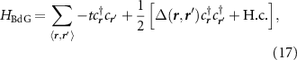
We discuss a pairing mechanism in interacting two-dimensional multipartite lattices that intrinsically leads to a second order topological superconducting state with a spatially modulated gap. When the chemical potential is close to Dirac points, oppositely moving electrons on the Fermi surface undergo an interference phenomenon in which the Berry phase converts a repulsive electron–electron interaction into an effective attraction. The topology of the superconducting phase manifests as gapped edge modes in the quasiparticle spectrum and Majorana Kramers pairs at the corners. We present symmetry arguments which constrain the possible form of the electron–electron interactions in these systems and classify the possible superconducting phases which result. Exact diagonalization of the Bogoliubov-de Gennes Hamiltonian confirms the existence of gapped edge states and Majorana corner states, which strongly depend on the spatial structure of the gap. Possible applications to vanadium-based superconducting kagome metals AV3Sb5 (A = K, Rb, Cs) are discussed.
Export citation and abstract BibTeX RIS

Original content from this work may be used under the terms of the Creative Commons Attribution 4.0 license. Any further distribution of this work must maintain attribution to the author(s) and the title of the work, journal citation and DOI.
1. Introduction
Since the discovery of high-temperature superconductors, investigations of superconducting instabilities driven purely by the repulsive Coulomb interaction have led to the discovery of numerous unconventional superconducting phases [1–8]. Among these, topological superconductors—hosting robust, zero-energy edge modes—have taken a key role in the pursuit of platforms for quantum computing [9–11]. Recently, a new classification of topological superconductors has emerged which relies on crystalline symmetries in addition to non-spatial ones [12–24]. These 'higher-order' topological superconductors host non-trivial boundary states with multiple dimensionalities: in two dimensions, the second-order topological superconducting phase hosts a gapped spectrum of propagating modes along the edge as well as zero-energy modes localized at the corners of the system in addition to a gapped bulk quasiparticle spectrum.
In the search for candidate materials hosting these phases, it is crucial to investigate the possible mechanisms that might give rise to them in physical systems, based on a microscopic analysis of the electron–electron interactions. In this work we describe an approach to interactions in two-dimensional materials with Dirac points that naturally leads to a second order topological  superconducting phase, arising past a critical doping for arbitrarily weak values of the repulsive Coulomb interaction. Our analysis is performed in the weak coupling regime, in which Stoner instabilities and correlated insulating states are absent, but the effects we describe dominate in materials where the atomic orbitals are strongly localized, which distinguishes our theory from those previously used to study graphene.
The Coulomb repulsion is converted into an attraction via destructive interference for certain scattering channels near the Dirac points which originate from the Berry phase, causing the formation of Cooper pairs to lower the correlation energy. Thus, our theory relies on Dirac Fermi surfaces, a scenario distinct from tuning the Fermi level to a nesting density or van Hove singularity, commonly studied as an explanation for superconductivity [25–31]. In contrast to previously studied mechanisms for higher order topological superconductivity, we also do not require proximitization to an existing superconductor [32–41], negative-U Hubbard interactions [42], or bosonic fluctuations [43].
This pairing mechanism was previously studied in the context of an artificial honeycomb lattice [44]; here we classify the resulting superconducting states and demonstrate their topological properties. Our results follow from general symmetry considerations, but we will present specific results for kagome and honeycomb lattices. In section 2 we discuss Hubbard-like models of these systems, presenting the most general set of interactions consistent with the lattice symmetries and enumerating the possible superconducting states which result. In section 3 we discuss how the superconducting instabilities are affected by screening effects. In section 4 we perform exact diagonalization of the Bogoliubov-de Gennes Hamiltonian describing the superconducting states, confirming the existence of edge and corner modes for samples whose edge respects the point group symmetry of the lattice. We conclude with a discussion of candidate materials, and suggest the mechanism can explain recently observed superconductivity in vanadium-based kagome metals AV3Sb5 (A = K, Rb, Cs), where superconductivity appears to be unconventional but correlations are weak [45–51].
2. Superconducting instabilities in Dirac materials
We investigate the pairing instabilities of a two-dimensional lattice with hexagonal symmetry hosting Dirac points at the K points, which we describe via an extended Hubbard model [52–54]
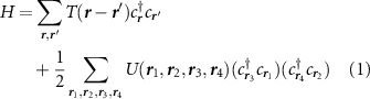
where  are two component spinors and the spin inner product is implied in the single particle and interacting terms in the Hamiltonian (1).
We choose lattice vectors  ,
,  , and specialize to lattices possessing
  symmetry, which consists of twofold and threefold rotations in the plane and mirror reflections about the x and y axes. We only consider models without spin-orbit interaction, thus we may choose a basis of Wannier orbitals so that
  and
and  are real. The Hamiltonian is invariant under SU(2) spin rotations and possesses a time reversal symmetry satisfying
  , which is identical to complex conjugation in the coordinate representation. For the remainder of this paper we denote the time reversal operation which leaves spin unaffected by
  .
.
The resulting band structure features Dirac points at the K and K' points, which we distinguish by a valley index  . The eigenstates of the single particle Hamiltonian may be classified by their eigenvalues
  under threefold rotations, where
  . We shall refer to the α degree of freedom as pseudospin. At the Dirac points there are four degenerate energy eigenstates
  which transform into one another under time reversal, twofold rotations and mirror symmetry. We shall introduce the Pauli operators
  acting on the valley and pseudospin degrees of freedom. The degeneracy of the α eigenstates at each valley is protected by either Mx
or
acting on the valley and pseudospin degrees of freedom. The degeneracy of the α eigenstates at each valley is protected by either Mx
or  . We obtain the following representation of crystal symmetries:
where φI is a phase which generally depends on the lattice and the chosen center of inversion.
Doping slightly above the valleys  , the Fermi surface consists of two circular pockets surrounding the K points with Fermi momenta
  , with the single particle energy eigenstates formed from linear combinations of the pseudospin basis states (i.e. eigenstates of threefold rotations). By obtaining the band structure of (1) and projecting the interactions onto states near the Dirac points, we obtain a quantum field theory describing interaction processes close to the Fermi level which accounts for the τ, α and spin (s) degrees of freedom and may be formulated using an eight-component local field operator
  . The most general Hamiltonian density consistent with the symmetries (2) is of the form
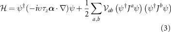
where we have expanded the interaction in the adjoint basis consisting of products  , and
, and  are constants which may be obtained by projecting the extended Hubbard interactions (1) onto the pseudospin and valley eigenstates. As we show in the
  . The Hamiltonian must transform as a scalar under the spatial symmetries (2) which implies that
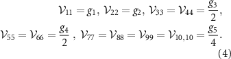
  is a diagonal matrix. There are only five independent coupling constants
  , which we relate to the interaction matrix
  by
by
In addition to a density–density interaction g1, the interactions involve valley-conserving ( ) and valley-mixing (
 ) mass operators. The remaining six operators are conserved SU(2) valley currents which can be expressed as products of the valley operators
  and the electric current
  .
.
The relation between the coupling constants gi
appearing in the field theory (3) and the extended Hubbard model parameters  for the kagome and honeycomb lattices are given in table 1. We denote the three sublattices of the kagome lattice
  , and the two sublattices of the honeycomb lattice by
  . We list only interactions involving nearest neighbors, and denote the interactions in which the lattice coordinates
  exist on the
  sublattices by
  . In the kagome lattice, each site has two nearest neighbors in each of the other sublattices, and in the honeycomb lattice, each site has three nearest neighbors in the other sublattice.
Table 1. The relations between coupling constants (3) and the extended Hubbard model parameters (1) for the Kagome and honeycomb lattice with couplings involving nearest neighbors. We denote  where
where  are sites in sublattices
  separated at most by a nearest neighbor bond.
| Kagome | Honeycomb | |
|---|---|---|

|

|
|

|

|
|

|
|

|

|
|

|

|

| UAAAA |
The eigenstates of the Dirac Hamiltonian in the upper band are given by  . Evaluating the Born amplitudes from (3) we find that the scattering vertex
  in the Cooper channel is given by
where θ is the scattering angle. BCS theory predicts that superconducting pairing occurs when the scattering amplitude between Cooper pairs is negative, i.e. for attractive scattering. For pairing of electrons within the same valley τ this corresponds to  , while pairing of electrons in opposite valleys requires the symmetrized amplitudes
  or
or  . The critical temperature is given

where  for intravalley pairing or
  for intervalley pairing, and
  is the density of states per spin per valley at the Fermi level.
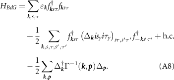
In order to investigate the physical features of the condensate we introduce the mean field Hamiltonian
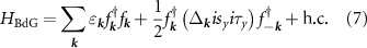
where  is the creation operator for a Dirac fermion in the upper band and
  is the superconducting gap matrix (spin and valley indices are implied). Accounting for spin, valley and angular momentum structure, there are eight possible superconducting phases, which we list in table 2 along with the corresponding scattering amplitude.
Table 2. Superconducting phases for 2D Dirac fermions in lattices with  symmetry. First column: gap structure, second column: order parameter, third column: coupling constant which determines Tc
via equation (6), in terms of coupling constants in the Hamiltonian equation (3), fourth column: Altland–Zirnbauer class.
symmetry. First column: gap structure, second column: order parameter, third column: coupling constant which determines Tc
via equation (6), in terms of coupling constants in the Hamiltonian equation (3), fourth column: Altland–Zirnbauer class.
| Gap structure | Δ | λ | AZ class |
|---|---|---|---|
| Intervalley, spin singlet, s-wave | τz |
| CI |
| Intervalley, spin singlet, p-wave |

|
| C |
| Intervalley, spin triplet, s-wave |

|
| BDI |
| Intervalley, spin triplet, p-wave |

|
| D |
| Intravalley, spin singlet, s-wave |

|

| CI |
| Intravalley, spin singlet, d-wave |

|

| CI |
| Intravalley, spin singlet, mixed s/d-wave |
|

| C |
| Intravalley, spin triplet, p-wave |
|
| BDI |
The topological properties of the gaps are associated with their Altland–Zirnbauer class [55–57], which classifies mean field Hamiltonians based on time reversal, charge conjugation and chiral symmetries. For the spin singlet pairing phases,  , accounting for SU(2) spin rotation symmetry we find that the charge conjugation symmetry satisfies
  . In the case of spin triplet pairing, the spontaneous violation of SU(2) spin rotation symmetry fixes a direction
  , with the gap
  . As we show in the
  . We therefore conclude that the phases with spin singlet pairing are either in class CI or C, while those with spin triplet pairing are either in class BDI or D depending on whether the time-reversal symmetry of the normal state Hamiltonian survives in the condensed phase. Consulting the periodic table of topological invariants [57], we find that first order topological superconductivity is possible for the phases in which time reversal symmetry is spontaneously broken, i.e. those in class C or D, and possess a Chern number which counts the number of chiral modes propagating along the boundary and whose parity is equal to the parity of Majorana modes localized at a vortex. However, both the intravalley p-wave spin triplet, and intervalley s-wave spin triplet states are in class BDI. For the intravalley spin triplet phase, the gap is p + ip in one valley and p − ip in the other, preserving time reversal symmetry, and we refer to this as the
  phase. In these cases lowest order topology is absent while second order topology is possible [14, 16, 20]. These phases are indicated by the existence of Majorana corner states of definite spin protected by crystalline symmetries. In addition to the spinless time reversal symmetry operator satisfying
  , our system possesses a spinful time reversal symmetry
  satisfying
  which interchanges opposite spin blocks; thus corner modes occur in Kramers pairs. In section 4 we present exact diagonalization results which demonstrate that the intravalley
  spin triplet phase indeed possesses a second order topology.
We now apply our previous results to analyze the possibility of superconducting instabilities in the kagome and honeycomb lattices. The leading Hubbard interactions do not involve tunneling between sites, thus we only account for interactions  in (1) with
  . Denoting the parameter λ in (6) by λ1 for intervalley s-wave spin triplet pairing, λ2 for intervalley p-wave spin triplet pairing and λ3 for intravalley p-wave spin triplet pairing, we find for the kagome lattice
where Ω is the area of the unit cell and
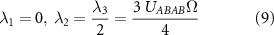
for the honeycomb lattice.
In the limit  the scattering amplitudes for all three spin triplet instabilities vanish for both lattices, implying that the system approaches a critical point for the onset of triplet superconductivity, including for the topologically nontrivial phases. The vanishing of the scattering amplitude in the p + ip and
  channels is a consequence of the Dirac nature of the scattering states, and can be understood as follows: the components of the wavefunction in the pseudospin and valley basis have momentum-dependent phase factors which are a manifestation of the Berry phase surrounding the Dirac points. Despite our model only containing local interactions, upon projecting the Dirac wavefunction onto the interactions in (3) we find that the Berry phase gives rise to p + ip scattering amplitudes which are essential to obtain a nontrivial topology. The pseudospin and valley dependence of the operators Ja
allows some gi
to contribute to the partial wave amplitudes λ with negative signs, as can be seen in table 2. This causes destructive interference between the contributions to the scattering amplitude with distinct pseudospin and valley structure—i.e. the gi
. In the scattering channels which give rise to the topological phases, the contributions from different gi
sum to zero, leading to a total cancellation of the on-site Coulomb repulsion.
channels is a consequence of the Dirac nature of the scattering states, and can be understood as follows: the components of the wavefunction in the pseudospin and valley basis have momentum-dependent phase factors which are a manifestation of the Berry phase surrounding the Dirac points. Despite our model only containing local interactions, upon projecting the Dirac wavefunction onto the interactions in (3) we find that the Berry phase gives rise to p + ip scattering amplitudes which are essential to obtain a nontrivial topology. The pseudospin and valley dependence of the operators Ja
allows some gi
to contribute to the partial wave amplitudes λ with negative signs, as can be seen in table 2. This causes destructive interference between the contributions to the scattering amplitude with distinct pseudospin and valley structure—i.e. the gi
. In the scattering channels which give rise to the topological phases, the contributions from different gi
sum to zero, leading to a total cancellation of the on-site Coulomb repulsion.
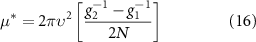
An additional negative contribution to the scattering amplitude which can overcome the weak nearest neighbor repulsion would result in superconductivity. One interesting scenario would be a weak electron-phonon interaction, which in our case could drive the instability to an unconventional spin triplet state, rather than the spin singlet state which normally results. In the next section, however, we will show that even in the absence of additional attractive interactions, a negative contribution to the nearest neighbor repulsion arises as a result of overscreening. All three triplet amplitudes become negative if the bare nearest neighbor repulsion is sufficiently weak, and the density is sufficiently high.
3. Screening effects
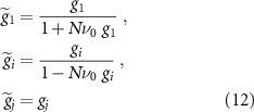
We now consider how gi
are modified by screening processes. We show these effects here analytically in the random phase approximation (RPA), equivalent to taking the limit of large N where N = 4 is the degeneracy of the Dirac points [59–62]. This analysis was performed for the special case of an artificial semiconductor honeycomb lattice in [44]; we extend this analysis to encompass generic Dirac materials satisfying  and time-reversal symmetry, which may be described by the Hamiltonian (3). The RPA results in replacing the interaction constants
  in (3) with screened frequency and momentum dependent couplings, which are determined by the RPA equation
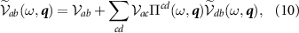
where  is a generalized polarization operator. These represent the susceptibility of the system to a perturbation
  , and are calculated in the
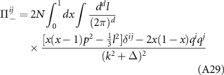
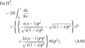
Accounting for the frequency and momentum dependence of the screened scattering vertex, solution of the Eliashberg equations gives the critical temperature

where  is the RPA renormalised λ of table 2 obtained from interactions between electrons on the Fermi surface and Λ is a frequency cutoff determined by scattering processes away from the Fermi surface; explicit calculation (discussed in the
  .
.
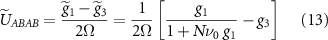
Scattering on the Fermi surface corresponds to the range of momentum and frequency transfer  , ω = 0. In this range the polarization operators are constant, and
  is simply given by the previous expressions λ (table 2) evaluated with screened couplings
  at
at  . We have studied the screening of the interactions g1 and g2 in a previous paper [44], and found that g1 is reduced while g2 is enhanced as the chemical potential is increased. We can explain the qualitative effects of static and homogeneous screening on the interactions on general physical grounds. The coupling g1 is screened by the long wavelength density–density response, which as usual weakens g1 with increasing chemical potential. The intra and intervalley mass couplings g2 and g4 are screened via the polarization operator associated with the response of the system to an external perturbation
  which gap the Dirac spectrum. This perturbation lowers the energy of negative energy states and increases the energy of the positive energy states. The response of the occupied negative energy states below the Dirac point is divergent and may be fully subtracted by regularization—the result of which is that g2 and g4 should be replaced by reduced interaction constants which are different from those provided in table 1; thus within the Dirac model the only physically significant effect of screening is the increase in energy of the occupied positive energy states which grows stronger with increasing chemical potential. The interactions
  are valley current interactions and the polarization operators responsible for their screening also contain a UV divergent part which may be subtracted by replacing the bare interaction constants with reduced values, and after this subtraction are unscreened due to a Ward identity. Explicitly, we find in RPA
where  and
and  . This results in replacing the nearest-neighbor coupling with a screened value,
  in the relations in table 1, equations (8) and (9). The screened nearest neighbor interaction is given by
for the kagome lattice and
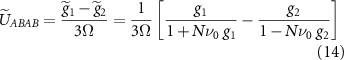
for the honeycomb lattice. For sufficiently large ν0, we find that  , resulting in superconductivity, and the dominant instability occurs in the intravalley, p-wave, spin triplet channel. This occurs for
  with the critical value
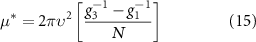
for the kagome lattice and
for the honeycomb lattice.
The Dirac theory is only applicable up to a cutoff beyond which the electronic dispersion becomes nonlinear. Our analysis predicts a superconducting instability when the critical doping  lies within the regime where Dirac theory is justified. In the limit
  or
or  respectively for the kagome and honeycomb lattices, the critical doping becomes infinite. We therefore require significant pseudospin dependent couplings, which are suppressed when the atomic orbitals are delocalized.
So far, we have neglected the long ranged part of the Coulomb interaction, which provides weak couplings between sites with large separation. This may be accounted for by replacing  with its screened value at
  ,
,  , and simply results in a shift of the critical doping to higher values.
4. Topological edge and corner modes
Our RPA results show that the dominant superconducting instability for both the honeycomb and Kagome lattice is the intravalley p–wave spin triplet phase, with gap structure  . This gap possesses a number of unconventional features that distinguish it from the superconducting phases more commonly studied in either high-Tc
superconductors or Dirac materials. The gap exists at both K points and has a
. This gap possesses a number of unconventional features that distinguish it from the superconducting phases more commonly studied in either high-Tc
superconductors or Dirac materials. The gap exists at both K points and has a  wave angular structure, which points to the presence of a π–Berry phase in two-particle scattering from which superconducting pairing originates. However, the winding of the gap is opposite in the two valleys, with the superconducting order parameter at the two K points being related to each other by complex conjugation. As a result, the usual topological features associated with chiral p-wave superconductors are strongly modified. We may view the phase as consisting of four copies of a topological p + ip superconductor [10], one per spin and valley species, with the gaps at opposite valleys possessing topological invariants of opposite sign. This results in a topologically trivial superconductor according to the Altland–Zirnbauer classification. However, in the presence of crystalline symmetries, a second order topology emerges which is characterized by anomalous corner modes.
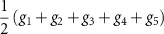
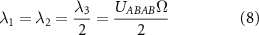
In the intravalley paired state, Cooper pairs carry a finite quasimomentum, and as a result the gap is spatially modulated, forming a pair density wave which is commensurate with the lattice with a periodicity of three unit cells [63–70]. The condensate possesses a U(1) order parameter φ associated with the spatial position of the pair density wave and does not couple to the electromagnetic field; the system also exhibits Goldstone modes associated with fluctuations of φ, which are physically the sliding modes of the pair density wave. The spatial modulation of the gap spontaneously breaks the crystalline symmetries of the normal state except at special values  ,
,  ; at these values the gap may be classified according to a second order topological invariant which predicts the number of Majorana corner modes of a finite sample of the superconductor which preserves the crystalline symmetries.
We study the topology of the  intravalley spin triplet phase via the bulk boundary correspondence for higher order topological superconductors, and identify the anomalous boundary physics in hexagonal superconducting flakes. By choosing a spin quantization axis which is aligned so that
  , we find that pairing occurs between electrons with both spins aligned either along the z or −z axis. Thus the pairing term may be decomposed into a sum of two spin sectors. We derive the topological features of the superconducting state by analyzing the spinless Hamiltonian corresponding to pairing within a single spin sector. In order to make numerical diagonalization easier we employ a simplified form of the gap function in which we only include nearest neighbor pairing and hopping terms. In the
  momentum space structure. The spinless mean field lattice Hamiltonian which results is
where 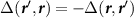 , and
, and
for the kagome lattice, and
for the honeycomb lattice, and we distinguish the parameter  from the bulk gap Δ.
We present exact diagonalization results for the kagome and honeycomb lattices in figures 1 and 2 respectively. We have calculated the spectrum for all values of φ, however the topological classification must be performed at the values  for which the gap obeys a twofold rotation symmetry. We have performed calculations for a variety of edge geometries, and in each case we preserve the twofold rotational symmetry of the bulk. In a number of cases we observe a gapless edge spectrum for all values of φ. This occurs for the geometries shown in the last two rows of figure 1 and the last row of figure 2. These surfaces states are remnants of the chiral Majorana edge modes expected from the Read-Green model [10] which are the most easily identifiable manifestions of the chiral p-wave nature of the gap. For other edge terminations, however, the edge spectrum is gapped, indicating that the gapless edge modes are not topologically protected, which is consistent with the fact that, since our gap lies in class BDI, it cannot possess a first order topological invariant. For the other edge terminations, we find that at
  , the edge states are gapped, and six zero energy modes appear within each spin sector which are localized at each of the corners of the flake, forming the three lowest modes within the quasiparticle spectrum of a single spin sector highlighted in red in figures 1, 2(c), (f) and (i). This occurs for both the honeycomb and kagome lattices. At φ = 0, we either find no Majorana zero modes when the edge spectrum is gapped or a gapless edge spectrum. This allows us to conclude that both the honeycomb and kagome lattices are in a second order topological phase for
  and trivial for φ = 0. We note that, since our results are for a spinless model obtained after performing a spin decomposition of the mean-field Hamiltonian, the Majorana zero modes appear as Kramers pairs. Since pairing occurs between electrons with parallel spin, the Majorana modes individually possess definite spin, and are protected against hybridization by a spinful time reversal symmetry
  .
.
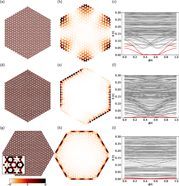
Figure 1. Results of the exact diagonalization of the Bogoliubov-de Gennes Hamiltonian within a single spin sector for hexagonal flakes of a kagome lattice of three different geometries. The leftmost figures show the spatially modulated pairing between nearest neighbors for  . The color of the bonds between neighboring sites
  shows the value of the gap function
  according to the color scale. The inset of the bottom left figure depicts a zoom into the bulk of the lattice with the unit cell boundary indicated by the thin lines. The central figures show the wavefunction densities of the three lowest quasiparticle modes. The rightmost figures show the quasiparticle spectrum as a function of the pair density wave parameter φ. The three lowest quasiparticle modes are indicated in red. For the exact diagonalization we use the parameters
  .
.
Download figure:
Standard image High-resolution image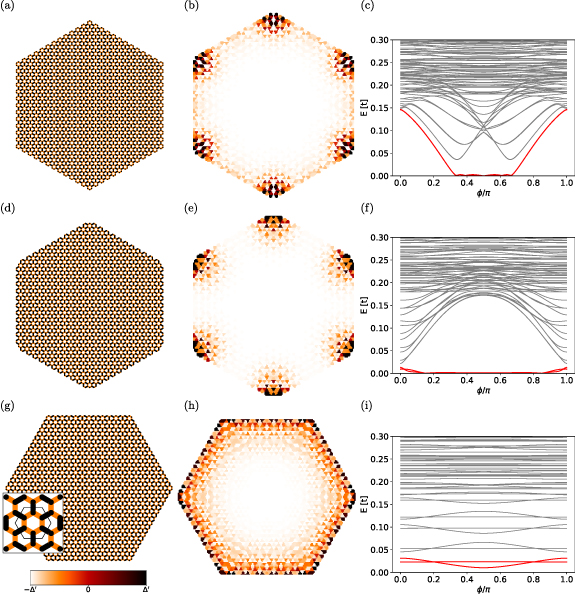
Figure 2. Results of the exact diagonalization of the Bogoliubov-de Gennes Hamiltonian within a single spin sector for hexagonal flakes of a honeycomb lattice of three different geometries. The leftmost figures show the spatially modulated pairing between nearest neighbors for  . The color of the bonds between neighboring sites
  shows the value of the gap function
  according to the color scale. The inset of the bottom left figure depicts a zoom into the bulk of the lattice with the unit cell boundary indicated by the thin lines. The central figures show the wavefunction densities of the three lowest quasiparticle modes. The rightmost figures show the quasiparticle spectrum as a function of the pair density wave parameter φ. The three lowest quasiparticle modes are indicated in red. For the exact diagonalization we use the parameters
  .
.
Download figure:
Standard image High-resolution imageSince the boundary modes in a higher order topological phase require crystalline symmetries, they are not protected against local perturbations. The robustness of the bulk-boundary correspondence in the presence of crystalline symmetry breaking therefore provides an important, general question for systems exhibiting higher order topology. In our examples, for general values of the pair density wave order parameter φ, all the point group symmetries of the normal state are spontaneously broken by the pairing term except for mirror reflection about the x axis, which is preserved due to the fact that the phase  of the pair density wave does not depend on the y coordinate. However, at discrete values
  , the superconductor recovers a twofold rotational symmetry. The parameter φ allows continuous tuning of the system between a second order topological phase at
  and a trivial phase at
  . We observe, despite the breaking of crystalline symmetries, that the anomalous corner modes persist and remain exponentially close to zero energy in a finite region of values around
  up to a critical value
  at which the edge gap closes. The corner modes are protected by both the bulk and edge gap, and thus persist even when the point group symmetry is weakly broken [13, 14].
The anomalous corner modes coexist with a gapped edge spectrum. This originates from the  nature of the gap, which provides a 1D boundary superconductor for each copy of the Moore-Read model existing in each spin and valley species. The manifestation of the bulk second order topology is shadowed by the behavior of the boundary superconductor: for certain edge terminations, the edge modes remain anomalous due to symmetries along the edge which forbid their hybridization. In particular, for the bottom geometries of figures 1 and 2, the system possesses a mirror symmetry at
  that prohibits the counterpropagating chiral Majorana modes from gapping out. In this case, the edge states are anomalous and associated with a bulk crystalline symmetry protected topological phase protected by mirror symmetry. For other edge terminations, mixing of the chiral modes between opposite valleys along the same edge occurs, and the edge spectrum is gapped. Interestingly, the emergence of anomalous corner modes in this situation is not general but depends on the value of φ.
We may make an interesting comparison to the p + ip intervalley spin triplet phase, which is subleading in our analysis in the regime where the onsite couplings dominate over the nearest neighbor couplings, but may arise as the dominant instability for models with more complicated lattice interactions. In this case, pairing occurs between the electron pockets surrounding opposite valleys, and the order parameter spontaneously chooses a winding number corresponding to either p + ip or p − ip pairing. Time reversal symmetry is broken, which puts the superconductor in class D, rather than BDI as in the intravalley case. This phase possesses a Chern number which leads to a gapless, anomalous edge spectrum. In a separate study, we show that this phase may become dominant when spin orbit coupling is present, and analyze the topology of this phase in detail [71].
5. Discussion
Our results show that the first order topological p + ip and second order topological  superconducting states emerge naturally in the presence of Dirac points near the chemical potential. While in a previous study we explored the pseudospin pairing mechanism giving rise to a
  instability in a semiconductor-based artificial honeycomb lattice within the RPA [44], in this work we have extended our analysis of the pairing mechanism to generic lattices satisfying
  symmetry and shown that this instability is not specific to any lattice structure but rather emerges due to the universal properties of the Dirac fermion excitations in these materials. We have illustrated that both the Berry phase and screening effects underlying the pairing mechanism are active in kagome lattices, and presented exact diagonalization results which demonstrate the striking similarity between the boundary physics in kagome and honeycomb lattices, which result from the fact that they possess identical topological properties.
In addition to the  phase, the intervalley p + ip and s-wave phase are possible, but are subleading in our analysis. The intervalley p + ip is a first order topological supercondutor with protected edge modes; the mechanism we describe here therefore can also result in first order topological superconductivity. Unlike the p-wave states, the s-wave state is protected against the effects of weak disorder by a generalized Anderson's theorem, so this state might posses a higher Tc
than the topological phases in a sufficiently disordered system. In a separate study, we also suggest that these two phases may arise due to spin–orbit coupling and study their properties in detail [71].
phase, the intervalley p + ip and s-wave phase are possible, but are subleading in our analysis. The intervalley p + ip is a first order topological supercondutor with protected edge modes; the mechanism we describe here therefore can also result in first order topological superconductivity. Unlike the p-wave states, the s-wave state is protected against the effects of weak disorder by a generalized Anderson's theorem, so this state might posses a higher Tc
than the topological phases in a sufficiently disordered system. In a separate study, we also suggest that these two phases may arise due to spin–orbit coupling and study their properties in detail [71].
We call attention to a number of relevant features of this mechanism: (i) the mechanism can be applied for weak repulsive interactions, so strong correlations are not necessary, (ii) superconductivity appears beyond a critical doping beyond the Dirac points, at which the screening effects become strong enough to give rise to a net attraction, (iii) the electronic origin of the pairing means the cutoff which determines Tc is the Fermi energy rather than the Debye frequency, (iv) superconductivity is more pronounced in systems with localized orbitals.
Superconductivity has recently been discovered in quasi-2D vanadium-based kagome metals AV3Sb5 (A = K, Rb, Cs) [45, 48]. The agreement between DFT calculations of the bandstructure and ARPES suggests that these materials are weakly correlated, an interpretation also supported by the results of DFT/DMFT calculations [45, 72, 73]. The Fermi surface contains pockets surrounding the Dirac points, a pocket surrounding the Γ point, and nearly-hexagonal Fermi contours [74]. Superconductivity exists alongside density wave order which sets in at a higher temperature and appears to compete with superconductivity [75–81]. STM and Josephson STS measurements suggest a spatially modulated superconducting gap [50] and zero bias peaks inside magnetic field-induced vortex cores are suggestive of Majorana bound states [51]. These materials also show signs of a phase transition between two distinct superconducting states as a function of doping [82].
Given that phonons appear unable to account for the measured Tc
[50, 73] and yet the materials appear to be weakly correlated, we propose that our mechanism might provide a partial explanation for superconductivity in kagome metals, in contrast to existing theoretical proposals which attribute superconductivity to the effects of nesting or competing density wave order [83–85]. In this interpretation, superconductivity originates from the Dirac-like Fermi surfaces and is not directly related to the observed charge density wave (CDW) order [75], which is potentially due to the nested portions of the band structure near the Fermi level. Due to the presence of multiple Fermi surfaces as well as Fermi surface reconstruction due to CDW order, our theory does not fully incorporate all the possible interactions. Given the apparent phase transition between two superconducting phases as doping is varied, we suggest that our theory may describe one of the observed phases, with different effects responsible for the other. Our theory can also not explain the observed periodicity of the pair density wave, however it is possible that this discrepancy is related to the reconstruction of the Fermi surface by the CDW, which would modify the spatial period predicted by our theory. Future experiments could look for evidence of the edge or corner modes present in the p + ip and  phases [23, 24], probe the spin structure of the gap through NMR or further investigate the real space structure of the superconducting gap as a function of doping/pressure.
Additional kagome systems have recently been discovered to host superconductivity, and might also be possible candidates for the pseudospin mechanism, including bilayer kagome systems [86], ferromagnetic kagome metals [87], and lanthanum-based materials [88]. Superconductivity has also been seen in Dirac surface states of doped topological insulators [89–93], which might also be explained by this theory. In materials such as transition metal dichalcogenides like MoS2 and MoTe2, and few-layer stanene [94], the presence of spin orbit interactions gaps the Dirac points and/or introduces a valley-Zeeman field, but the Dirac physics persists nonetheless. In a separate study, we have examined the effects of spin–orbit coupling on the possible superconducting states, and find that the pseudospin mechanism results in topological superconductivity in these systems as well [71]. Our mechanism may also play a role in the observed superconducting phases in Moiré systems such as twisted bilayer/trilayer graphene [95–98]. These systems exhibit honeycomb/kagome superlattices hosting Dirac points, however, while our theory is expected to be applicable, the interaction structure is significantly more complicated than for the monolayer honeycomb or kagome materials we have investigated. As a general guiding principle, promising candidate materials for the pseudospin mechanism are those with strongly localized orbitals—which lead to larger values of the couplings gi
and lower values of the critical doping  —and larger Dirac-like Fermi surfaces—which enhance the screening effects.
Acknowledgments
The authors thank B Ortiz, P Brouwer, M Scheurer and P Kotetes for helpful discussions. M G acknowledges support by the European Research Council (ERC) under the European Union's Horizon 2020 research and innovation program under Grant Agreement No. 856526, and from the Deutsche Forschungsgemeinschaft (DFG) Project Grant 277101999 within the CRC network TR 183 'Entangled States of Matter' (subproject A03 and C01), and from the Danish National Research Foundation, the Danish Council for Independent Research | Natural Sciences. H D Scammell acknowledges funding from ARC Centre of Excellence FLEET. T L acknowledges support from the DFG within the CRC network TR 183.
Data availability statement
All data that support the findings of this study are included within the article (and any supplementary files).
Appendix
Appendix. Symmetry relations for the effective field theory
We may explicitly derive the interaction parameters  in equation (3) of the main text by projecting the extended Hubbard interactions onto the valley and pseudospin eigenstates
  . We find
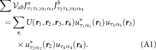
The Hubbard interactions may be expressed in terms of the Wannier orbitals  (with x being a 3D coordinate vector) via
where  is the Coulomb interaction, and we have chosen the Wannier orbitals to be purely real. The interactions thus satisfy
  .
.
We may use the representation of time reversal symmetry (equation (2) in the main text)  with
with  to derive a relation
Applying this to the factors  and
and  in (A1) we find
We may express this in the form
Since the adjoint basis elements Ja
are Hermitian and transform with definite sign under time reversal,  , we find that
  for any operator Ja
which is odd under time reversal.
for any operator Ja
which is odd under time reversal.
We may derive further symmetry constraints using the relations

where Λ is a symmetry operation acting on coordinates and  is its unitary representation. Applying a simultaneous transformation
  in (A1) we find
Since there always exists a symmetry operation under which Ja
and Jb
transform with opposite signs unless a = b, we find that  is a diagonal matrix.
Appendix. Landau–Ginzburg analysis of the superconducting gap symmetry
The generic mean field Hamiltonian to account for all pairing possibilities, in the upper band, is
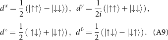
The gap takes any of the forms presented in table 2, which contains the valley, spatial and spin structure. The spin structure employs standard notation of dµ -vectors;
The analysis presented in the main text states that the gap functions can be chosen as simply one of the possible degenerate sets; for the gap structure discussed in section 4 it is important that we can choose the d-vector along one axis  , and that a non-unitary choice of
  is energetically penalized. We explicitly show that this is the case below. We compute the free energy to quartic order from (A8), and find
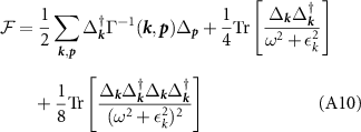
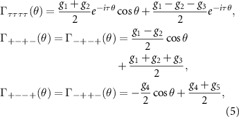
where Γ are the Cooper channel Born amplitudes, explicitly given in (5), and the trace includes summation over momentum and frequency.
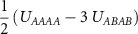
Each gap structure entering table 2 has a critical temperature set by the coupling λ, where  for intravalley pairing, while
  for intervalley pairing. We restrict our attention to work within each degenerate set of gaps separately. In most cases, the valley structure is trivially traced out—the free energy reduces to separate cases based on the overall spin degeneracy
  and degenerate chiral phase factors
  . Using this logic, there are only five distinct cases to consider
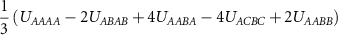
Case (iii) enumerates the two physically distinct valley structures that share the same spin structure and chirality, but themselves are not degenerate, i.e. have different Tc
. The differing valley structures of these gaps does not affect the contribution to  that is quartic in Δ; the valley structure enters through Γ and affects the value of Tc
but not the stability analysis. The brackets in (v) accounts for the four physically distinct gap structures which are degenerate, i.e. have the same value of λ and hence have same critical temperature, cf table 2. We combine these three gap functions into a vector
that is quartic in Δ; the valley structure enters through Γ and affects the value of Tc
but not the stability analysis. The brackets in (v) accounts for the four physically distinct gap structures which are degenerate, i.e. have the same value of λ and hence have same critical temperature, cf table 2. We combine these three gap functions into a vector  , which will use below in the free energy analysis.
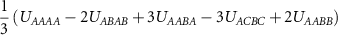
Evaluating the free energy to quartic order in the gaps,
with coefficients 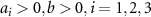 . We summarize the main conclusions:
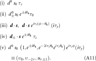
- Case (i) is a s-wave singlet paired state. The free energy straightforwardly establishes stability of this phase.
- Case (ii) corresponds to an intervalley p + ip state, in which electrons from opposite valleys pair with a definite chirality. From
![${\cal F}_2[ d^{\,0}_{\pm} s_0 e^{\pm i \theta_{\boldsymbol{k}}}]$](data:image/png;base64,iVBORw0KGgoAAAANSUhEUgAAAAEAAAABCAQAAAC1HAwCAAAAC0lEQVR42mNkYAAAAAYAAjCB0C8AAAAASUVORK5CYII=) , we find that coexistence of opposite chiralities is energetically penalized so that the system spontaneously chooses one chirality, e.g. , therefore breaking time reversal. This state exhibit first order topology with gapless edge states.
, we find that coexistence of opposite chiralities is energetically penalized so that the system spontaneously chooses one chirality, e.g. , therefore breaking time reversal. This state exhibit first order topology with gapless edge states. - Case (iii) concerns two triplet paired states for which the free energy has the same form; from we find that non-unitary paring is penalised, i.e.
d
is purely real (or purely imaginary); the
d
vector spontaneously chooses a direction, breaking spin SU(2) symmetry, but the condensate has vanishing magnetization. The two superconducting states included in this case are: intravalley , in which electrons undergo p + ip pairing in one valley and p − ip pairing in the other, and intervalley s-wave, in which electrons from opposite valleys undergo triplet s-wave pairing. Both states respect time-reversal symmetry.
- Case (iv) examines spin-triplet p-wave intervalley pairing. From , similar to case (ii), the resulting state spontaneously breaks time reversal symmetry, resulting in a first order topological p + ip state e.g. . As in case (iii), we again find the d-vector is purely real (or imaginary), and hence this state breaks time reversal symmetry but does not support a magnetization.
- Case (v) looks at a degenerate manifold of s-wave, , and a mixed state with s-wave in one valley and a pairing in the opposite valley, the latter of which breaks time reversal. The intravalley d-wave state is a superconductor—a time reversal invariant combination of d + id pairing in one valley, and d − id pairing in the other—and exhibits second order topology with gapless corner states.
![${\cal F}_2[ d^{\,0}_{\pm} s_0 e^{\pm i \theta_{\boldsymbol{k}}}]$](https://content.cld.iop.org/journals/2053-1583/9/1/015031/revision2/tdmac4060ieqn173.gif)

![${\cal F}_3[ \boldsymbol{d}\cdot \boldsymbol{s} ]$](https://content.cld.iop.org/journals/2053-1583/9/1/015031/revision2/tdmac4060ieqn175.gif)

![${\cal F}_4[ \boldsymbol{d}_\pm\cdot \boldsymbol{s} \ e^{\pm i \theta_{\boldsymbol{k}}} ]$](https://content.cld.iop.org/journals/2053-1583/9/1/015031/revision2/tdmac4060ieqn177.gif)


Appendix. Screened interactions
In this appendix we discuss the screened electron–electron interactions. We begin by presenting general expressions for the polarization operators, and making some general comments about regulating UV divergences in effective quantum field theories. We then explicitly calculate the intra and inter valley current-current susceptibilities. We present the formulae for the screened couplings, and plot the frequency dependence of the resulting scattering amplitudes for Cooper pairs. We conclude by discussing alternative regularizations for computing the susceptibilities.
Preliminaries
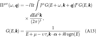
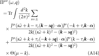
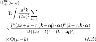
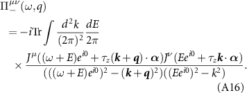
The RPA equations for the screened interactions are
where  is the polarization operator,
where the vertices 
 , as per section 4 of the main text. We choose units in which υ = 1, and upon performing the frequency integral by residues, manipulations presented in [44] result in
The first term—the interband polarization operator, denoted  —contributes when µ = 0, while the second term—the intraband polarization operator, denoted
  —only contributes when µ ≠ 0. Explicitly, we write
and
The polarization operator Π11 is the standard charge polarization operator for graphene [60, 61, 99], which describes the screening of the density–density interaction  . The function Π22 is the pseudospin polarization operator which describes the screening behavior of the pseudospin–pseudospin interaction
  which was first calculated in [44] (denoted there as
  due to different notation and a difference choice of basis for the pseudospin states). The remaining functions describe the screening of the intra and intervalley chiral currents. The current-current susceptibility for graphene has been discussed in [100–102], though to the best of our knowledge the intervalley current-current susceptibility has not been previously investigated. Below, it will be convenient for us to derive expressions for both functions, and present them in a form somewhat more general than those already in the literature.
All polarization operators may all be written in terms of four basic functions, for which we will introduce simple notation in what follows. Use the spacetime indices  where
where  , and denote Π22 as
  . Considering
  and
and  , i.e. the chiral current screening
  , we then write this function as
  and decompose into longitudinal and transverse parts:
The chiral current polarization operator obeys an important identity due to electromagnetic gauge invariance. In the Dirac theory, the electromagnetic current operator  so that the vector potential of electromagnetism
A
appears in the Hamiltonian as the perturbation
so that the vector potential of electromagnetism
A
appears in the Hamiltonian as the perturbation  . Gauge invariance, or equivalently the conservation of charge, can be shown to imply the Ward identity,

From this we find
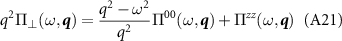
Combining these,

which gives us an expression for the longitudinal part of the current-current susceptibility in terms of the density-density response
Comparing our below results with the expression for Π00 cite [44] shows our expressions satisfy this relation. We shall also derive an expression for the transverse part of the susceptibility in the dimensional regularization scheme,
which therefore allows the current-current screening operator to be written entirely in terms of the density and pseudospin responses.
As is common quantum field theories, the polarization operators are formally divergent quantities and require regularization. However, the physical origins of the divergences and the effects of regularization differ between the polarization operators. The dimensional regularization scheme has the effect of simply setting all UV contributions to zero, leaving just the effects of those degrees of freedom in the Dirac effective theory near the K-points. Since actual materials are UV-completed by a lattice, placing the theory on a lattice is a more physical regularization scheme, and gives the physical relation between the numerical values of the couplings computed by band structure methods and the couplings in the effective theory.
Firstly, the charge susceptibility  obeys the exact compressibility sum rule,
  where ν0 is the density of states at the Fermi level, which means that cutoff-dependent quantities never appear in any sensible regularization scheme. For small frequencies and momenta, the regularized polarization operator must be the same as that calculated in dimensional regularization.
Second, the current susceptibilities  obey the Ward identity discussed above, as a result of the fact that
α
is the current operator in the Dirac theory, which also excludes cutoff-dependent contributions. However, away from the K-points, the current operator is no longer given by
α
, which will result in UV-dependent contributions to
obey the Ward identity discussed above, as a result of the fact that
α
is the current operator in the Dirac theory, which also excludes cutoff-dependent contributions. However, away from the K-points, the current operator is no longer given by
α
, which will result in UV-dependent contributions to  . In the lattice regularization scheme, this means that one can make changes to the lattice—for instance by modifying the dispersion near the Γ point—that will result in a different value for
  , but these UV-contributions originate from physics away from the Dirac point where the Ward identity applies. Similar to
  , for small frequencies and momenta, the regularized
  must be the same in lattice and dimensional regularization.
The pseudospin susceptibility  , by contrast, obeys no such constraint and receives a constant and negative cutoff dependent contribution in a lattice regularization. We may distinguish between two types of cutoff dependence—contributions which originate from physics near the Dirac point, and contributions which originate from physics away from the Dirac point. While only the latter affects
  , as we explained above, both types of UV-contributions appear in
  ; one way to see this is to use a hard cutoff Λ in the Dirac theory, where (restoring the Dirac velocity v) one finds
  . Thus by solely modifying physics near the Dirac point—for instance by changing the velocity—these UV contributions which originate from physics near the Dirac point are changed. As a result, these contributions which appear in a lattice regularization are important even at small frequencies and momenta, and are described in the main text.
When working with an effective field theory, one always performs calculations in terms of UV-independent quantities. However, if one wishes to perform a microscopic calculation of the couplings gi
in (equation 4)—by computing the wavefunctions of a material for e.g. through band structure diagonalization and then taking matrix elements of the Coulomb interaction—the couplings which appear in the effective quantum field theory will be related to those values through lattice regularization, in which  and
and  receive contributions from physics away from the Dirac point, and
  receives an additional constant contribution from physics near the Dirac point.
Intravalley current-current polarization operator
We now turn to a calculation of  . We begin by calculating the interband part through dimensional regularization, using the formulae
Focus first on the denominator in equation (A16). Using the Schwinger–Feynman parametrization,
we write
where we now use relativistic notation  ,
,  , and
, and  ,
,  . Shifting
  (bear in mind that this will affect the numerator as well), and Wick rotating
  , the expression becomes
The corresponding numerator (before Wick rotation) is
Now we substitute  with
with  and perform the pseudospin trace using the identity
where  . Using rotational symmetry to replace
  , we arrive at
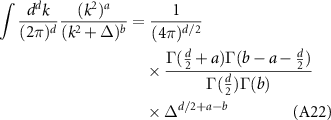
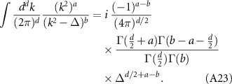
where we account for the valley and spin trace through a factor N = 4. Integrating using equation (A23), we find the imaginary part
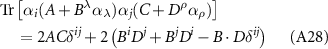
Using  , we arrive at
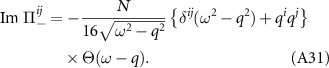
Similarly using equation (A22), the real part is calculated from equation (A29) to be

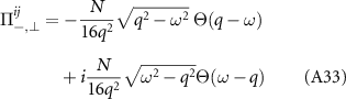
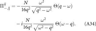
The functions  and
and  are respectively the transverse and longitudinal components of the polarization operator. From above, we see the their interband parts are
and
Calculating the density response  through the formalism above, one may see that the above expression for
  satisfies the Ward identity (A20).
Let us now perform the intraband calculation. The numerator in equation (A15) is evaluated using equation (A28), so that
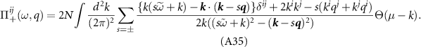
The denominator equals  . Shifting the angle of integration
  where
where  is the angle of the vector
q
, and denoting the angle of integration hereafter as simply θ, we have
is the angle of the vector
q
, and denoting the angle of integration hereafter as simply θ, we have  . Using the evenness of the denominator in θ, the numerator may be simplified to arrive at

where  . To proceed, we make use of the integral
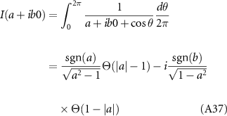
and the identities
Evaluating (A36), we define  and denote
  . Then
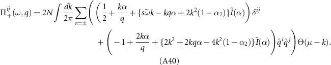
Making the substitution  , we get

We arrive at
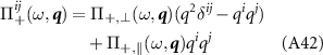
with
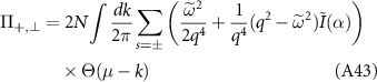
and
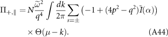
As stated earlier, the latter function is related to the density response through the Ward identity. Direct comparison with the appendix of [44] shows that the Ward identity is satisfied by the above expression. One also sees that the inter and intraband polarization operators separately satisfy equation (A21). In summary, one finds

with
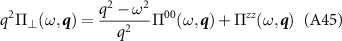
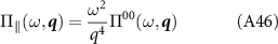
as claimed in the previous section.
Intervalley polarization operator
Taking  and
and  with
with 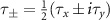 and performing the trace changes the sign of the terms containing factors of τz
. If we denote this intervalley polarization operator
and performing the trace changes the sign of the terms containing factors of τz
. If we denote this intervalley polarization operator  then one finds the simple result
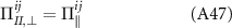
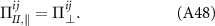
In other words, the transverse and longitudinal response are reversed between intra and intervalley. The same trace relations show that  , i.e. the screening of the operators
  is the same as that of
  .
.
Solution to the RPA equations in the onsite limit
We have the interactions
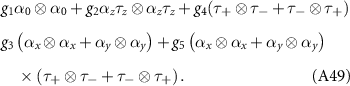
We consider the simple case of only onsite interactions, so only  ; in this limit one finds
  for the honeycomb lattice and
  for kagome lattices. In each case the RPA equations decouple, so that each gi
is screened separately. The result is the screened interactions:
for kagome lattices. In each case the RPA equations decouple, so that each gi
is screened separately. The result is the screened interactions:
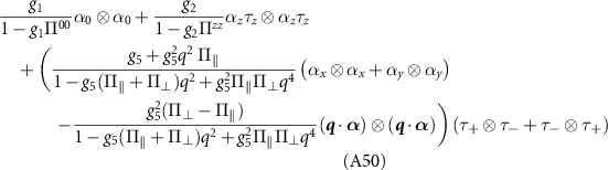
for the honeycomb lattice and
for the kagome lattice.
Cooper channel scattering amplitudes
On-site limit for honeycomb systems
For honeycomb systems, the  -wave scattering amplitude is
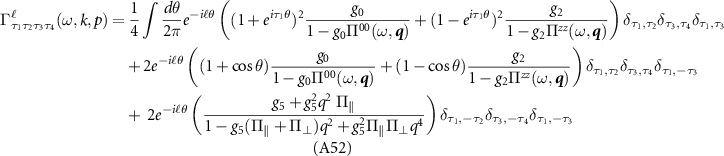
where  ,
,  .
.
On-site limit for kagome systems
For the kagome lattice we have
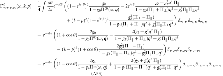
Eliashberg equations
Neglecting self-energy corrections, the linearized Gor'kov–Eliashberg frequency dependent gap equation is given
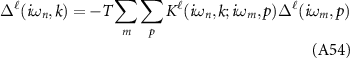
with the Eliashberg kernel,
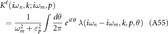
where  are the fermionic Matsubara frequencies [103–105]. The frequency dependent coupling
  is defined analogously to the static coupling in the main text:
  for intravalley pairing or
  for intervalley pairing. The functions Δ, K and Γ are tensors in spin and valley space—spin and valley indices are left implicit. The critical temperature can found by finding the value of T for which the above linear equation for Δ has an eigenvalue of
  . The zero temperature gap can also be found from solving

where  is the
  -wave coupling evaluated onshell,
  . These equations can be derived through general assumptions about the analytic behavior of the scattering amplitude Γ (see e.g. [103]). The requirements of unitarity and causality imply that as a function of frequency the amplitude must be analytic in the upper half plane, and that the amplitude has branch cuts corresponding to the threshold of particle-hole production. While Γ possesses singularities as a function of
  , these occur either for
  , which provides a negligible contribution, or close to the edge of the particle hole continuum
  , which is significant for a range of scattering angles
  which only becomes significant when
  .
.
As is shown by examination of the formulae in the previous subsection, the scattering amplitudes have a roughly step-like behavior. Below, we plot the p-wave inter and intra valley on-shell couplings— as well as
  —for the kagome and honeycomb lattices to illustrate this phenomenon. Treating the scattering amplitude as a step function in frequency space, the frequency dependent gap equation can therefore be straightforwardly solved as in the Anderson-Morel treatment of the electron-phonon problem [106], the result being a renormalized coupling appearing in the exponential form of Tc
and an effective frequency cutoff, c.f. the treatment in S3 of [44].
—for the kagome and honeycomb lattices to illustrate this phenomenon. Treating the scattering amplitude as a step function in frequency space, the frequency dependent gap equation can therefore be straightforwardly solved as in the Anderson-Morel treatment of the electron-phonon problem [106], the result being a renormalized coupling appearing in the exponential form of Tc
and an effective frequency cutoff, c.f. the treatment in S3 of [44].

Figure A1. The p-wave intravalley coupling function  , and s-wave intervalley coupling function
  for honeycomb (left column) and kagome (right column) systems in the onsite limit. We use fine structure constant
  , bare couplings
  , and for the intrarvalley coupling functions use
  and for the intervalley coupling functions
  . The scattering amplitudes have been regularized and smoothed to avoid singularities which are inessential to the solution of the gap equation, as discussed in the Appendix section "Eliashberg equations".
Download figure:
Standard image High-resolution imageAppendix. Real space form of the gap function

In this appendix we derive the real space form of the  gap function used for exact diagonalization in section 4. Starting with the momentum space mean field Hamiltonian, we have
where  creates an electron in the upper band,
  is an overall factor depending only on the magnitude k, φ is the phase of the pair density wave, and
  is a constant 3D vector with unit length. The normal dispersioon
  is spin independent, which allows us to perform a spin rotation so that
  , and the Hamiltonian decouples into two spin-diagonal terms,
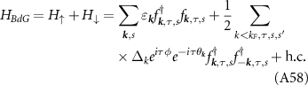
Since the Hamiltonian is a sum of independent spin blocks, we discard the spin index henceforth. We now convert this expression to real space, in which the Hamiltonian becomes
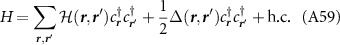
where  is the full electron creation operator (as compared to
  which creates an electron with momentum
k
in the upper band). We assume that the only hopping term present connects nearest neighbors, i.e. that
which creates an electron with momentum
k
in the upper band). We assume that the only hopping term present connects nearest neighbors, i.e. that  if
r
and
if
r
and  are nearest neighbors and zero else. It remains then to calculate the function
  . In momentum space, the pairing term for each spin block is given by
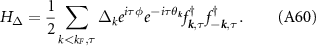
We relate the creation operator for the upper band to the full electron creation operator by
where  is the wavefunction for the upper Dirac band. Substituting this relation into the pairing term,
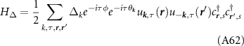
from which it follows immediately that

The upper band eigenstates of the Dirac Hamiltonian  are given in the coordinate representation in terms of the wavefunctions
  by
by
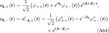
where  are periodic functions under lattice translations. Thus
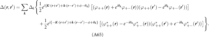
Performing the summation over k and introducing the functions
we find
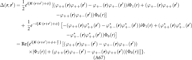
The function  is maximum for r = 0 and goes to zero over length scales
  while
while  is small for small r and increases to a maximum at
  . To simplify
  for the purposes of exact diagonalization, we will neglect the pairing correlations at large separations, discarding the term containing Φ1 and set
  with
with  being some average value. With these simplifications we finally arrive at the real space Hamiltonian
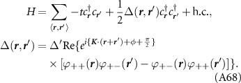
Note that  , and with t real, the Hamiltonian is invariant under complex conjugation, conforming with our claim in the main text that this superconducting phase lies in class BDI.
Below we present  explicitly for the honeycomb and Kagome lattices. The procedure is simply to calculate the eigenfunctions
  of the normal state Hamiltonians at the Dirac points, and insert into equation (A68).
Honeycomb lattice

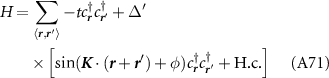
Kagome lattice
For the kagome lattice, we have
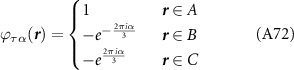
so the real space gap function is
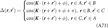
and hence
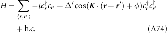
with the appropriate orderings of
r
and  to take account of the case with a relative π phase—as per equation (18).
Footnotes
- 6
We note that the pairing term only possesses U(1) spin symmetry, however the normal state dispersion retains its original SU(2) spin symmetry. It was noted in [58] that such a state generically falls in class D.