
Abstract
Shear-assisted liquid exfoliation is a primary candidate for producing defect-free two-dimensional (2D) materials. A range of approaches that delaminate nanosheets from layered precursors in solution have emerged in recent years. Diverse hydrodynamic conditions exist across these methods, and combined with low-throughput, high-cost characterization techniques, strongly contribute to the wide variability in performance and material quality. Nanosheet concentration and production rate are usually correlated against operating parameters unique to each production method, making it difficult to compare, optimize and predict scale-up performance. Here, we reveal the shear exfoliation mechanism from precursor to 2D material and extract the derived hydrodynamic parameters and scaling relationship that are key to nanomaterial output and common to all shear exfoliation processes. Our investigations use conditions created from two different hydrodynamic instabilities—Taylor vortices and interfacial waves—and combine materials characterization, fluid dynamics experiments and numerical simulations. Using graphene as the prototypical 2D material, we find that scaling of concentration of few-layer nanosheets depends on local strain rate distribution, relationship to the critical exfoliation criterion, and precursor residence time. We report a transmission-reflectance method to measure concentration profiles in real-time, using low-cost optoelectronics and without the need to remove the layered precursor material from the dispersion. We show that our high-throughput, in situ approach has broad uses by controlling the number of atomic layers on-the-fly, rapidly optimizing green solvent design to maximize yield, and viewing live production rates. Combining the findings on the hydrodynamics of exfoliation with this monitoring technique, we unlock targeted process intensification, quality control, batch traceability and individually customizable 2D materials on-demand.
Export citation and abstract BibTeX RIS

Original content from this work may be used under the terms of the Creative Commons Attribution 4.0 license. Any further distribution of this work must maintain attribution to the author(s) and the title of the work, journal citation and DOI.
1. Introduction
The potential for graphene and related two-dimensional (2D) materials to disrupt a vast range of technologies has brought the challenge of scalable material production into focus [1–3]. Their importance is underlined by the opportunity they provide to vastly improve, and create new technologies (batteries, capacitors, photovoltaics, membranes, flexible electronics, photonics, communications, etc) that can solve grand challenges across energy, sustainability and healthcare [3]. Material quality and morphology are influenced by the production method [4, 5], intrinsically linking the performance of technologies employing 2D materials to the synthesis route [6]. A prominent approach, with perhaps the most versatility, is liquid exfoliation [7]. Despite mass production being feasible, commercially available materials are incorrectly classified (few-layer graphene (FLG) vs nanoplatelets) and the quality is overwhelmingly sub-optimal at present [8]. While widespread control of quality can be supported through international standardization, many fundamental challenges must be solved if this, and application-specific materials by design, are to be realized. Controllable selectivity, reproducible quality, process scalability and high-throughput characterization techniques remain significant limitations from the lab to industrial scales [9–11]. These factors are interdependent, as quality control requires batch-to-batch monitoring and current 2D material characterization methods are too time-consuming and expensive for this purpose [8, 11]. The emphasis goes beyond graphene too, as other useful layered materials and van der Waals heterostructures are discovered and found to be exfoliable [2, 12].
Hydrodynamics are central in many nanomaterial exfoliation and dispersion processes that rely on shear-assistance [13–15]. Methods have been designed to exceed a minimum shear rate necessary to exfoliate layered materials [14, 16] using laminar [17], turbulent [18–21] and multiphase flows [13] in the search for higher yields and one-pass ink formulation. Even so, the yield of FLG with atomic layers less than ten, is typically single percentage levels [19]. Small gains in performance, through optimization of shear exfoliation conditions, would greatly benefit process output and resource efficiency, particularly at large scales. At the nanoscale, controlled separation of individual graphene sheets has been studied using molecular dynamics [22–24] and micromechanical models [25]. At micro- and macro-scales, scaling of production performance is typically based on empirical correlations fitted to operating parameters that are unique to the exfoliation method. While useful for assessing process sensitivity to independent input parameters, the local fluid mechanics and transport phenomena promoting exfoliation are concealed. Uncovering this is crucial, given the importance to exfoliation rates and for developing a framework to predict the scalability of processes without empirical data.
Here, we report the relationship between graphene production and the hydrodynamics of exfoliation. Using two different exfoliation methods to produce graphene, we find that strain rate distribution and precursor residence time are the dominant factors that govern nanosheet concentration scaling in shear-assisted exfoliation. In particular, this time parameter has been largely neglected and we show here that it plays a significant role in production output. We introduce an indirect reflectance spectroscopy method for monitoring the absorbance behavior of these dynamic, fluid dispersions in real-time, providing a solution amenable to Industry 4.0 [26]. We use this method to extract graphene concentration profiles from the multi-component mixtures (solvent, precursor and 2D material) during exfoliation. In doing so, we demonstrate real-time monitoring of 2D material production without the need for centrifugation and separation, saving hours of material post-processing and preparation time. Following this, we demonstrate control of average layer number on the fly, by applying known strain rates to FLG dispersions and simultaneously measuring multi-spectral features. Using low cost optoelectronics, our approach opens up 2D materials characterization to any individual, while also enabling control over the entire value chain to ensure minimal waste, maximum traceability, and on-demand materials by design.
2. Results and discussion
2.1. Scaling of concentration with hydrodynamics
We investigated the hydrodynamics of exfoliation in a general way, by considering two continuous exfoliation processes with different shear conditions. The first was based on turbulent Taylor–Couette flow (figure 1), and the second used laminar, thin film flow over a spinning disc (figure 2). Both generate high shear stresses in an exfoliation region labeled as Z1 in figures 1(A) and (B) and 2(A) and (B), and can produce 2D materials [13, 20, 21]. Both exfoliation experiments were designed to permit optical access for high speed imaging of the material flows while simultaneously producing graphene from graphite/N-methyl-2-pyrrolidone (NMP) dispersions (Materials and methods).
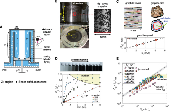
Figure 1.
Production of graphene using Taylor–Couette flow. (A) Schematic of the liquid exfoliation system. (B) Side view and top view images of the experimental device under exfoliation conditions (top left, bottom left). A snapshot of graphite microparticles dispersed in NMP during exfoliation and obtained using a high-speed camera (right). (C) Graphite particle tracks for  (top left). An optical microscopy image of a graphite particle and an illustration of changes to particle size with processing time (top right). Average graphite particle speed due to changes in the rotational speed of the inner cylinder (bottom). (D) Post-centrifugation graphene/NMP dispersions at increasing processing times from left to right (top image). Concentration of graphene with processing time for various operational speeds (bottom). (E) Scaling of graphene production with device hydrodynamics. Ci = 10 g l−1 in (B) to (E).
Download figure:
Standard image High-resolution image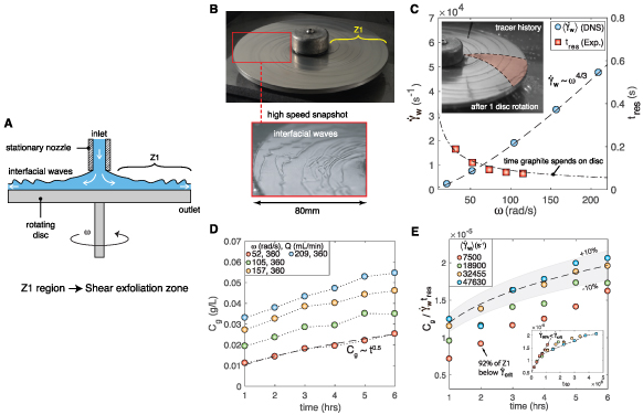
Figure 2.
Production of graphene using spinning disc flow. (A) Schematic of the liquid exfoliation system. (B) Image of the experimental device (top) and a high speed image showing the interfacial waves produced under exfoliation conditions (bottom). (C) Changes in strain rate and particle residence time with operating speed. Tracer history after one complete disc rotation (inset) (D) Concentration of graphene for various operational speeds. (E) Scaling of graphene production with device hydrodynamics. Note the abscissa is represented by time instead of No as in Taylor–Couette exfoliation (figure 1(E)). In the spinning disc device, graphite leaves Z1 without orbiting the disc (B, tracer history) and No
= 0. Inset plot shows  scaling time on disc speed,
  . Ci = 5 g l−1 in (D and E).
Download figure:
Standard image High-resolution imageIn the Taylor–Couette system, the precursor paths, speed, size and shape were measured with time (figures 1(B) and (C)). Samples were also taken during operation to obtain nanosheet concentration (figure 1(D)). The Taylor vortex zone (Z1) provides the conditions for exfoliation, and the fluid mixture exits through an inner cylinder zone (Z2). These vortices originate from centrifugal instabilities in the fluid gap between the concentric cylinders [27]. Z2 controlled concentration saturation by promoting sedimentation of graphitic material on the inside surface of the hollow inner cylinder at high speeds when the centrifugal force (Fc) dominates gravity (Fg). A scale analysis on the full force balance equation for a particle indicates that this occurs when  rad s−1, agreeing with the experimental observations of concentration saturation in figure 1(D) (see also section S6). This reduces the rate of production by reducing the amount of precursor material that gets circulated through the device. Prior to saturation, the linear part shows
  , indicating the effectiveness of both the high shear environment and the intense mixing characteristics of Taylor vortex flows. For high rotational speeds (
 rad s−1), a lower rate transition region exists between the initial linearly increasing concentration and the saturation condition at later process times. These varied linear to non-linear graphene concentration profiles were used to test the robustness of in situ production monitoring, discussed in section 2.3.
Dispersions of graphite particles in NMP (Ci = 10 g l−1) were continuously pumped through at a sufficiently low volumetric flow rate (325 ml min−1). This method maintained the Taylor vortex flow structure in the d = 2 mm fluid gap. We observed a rheoscopic behavior from the graphite/NMP mixture, where graphite flakes orient to the flow, revealing the hidden vortices in figure 1(B) as alternating dark–bright 'bands'. We confirmed this observation by recording the motion of individual precursor particles (movie S1 (available online at stacks.iop.org/tdm/8/025029/mmedia)). Using particle image velocimetry, and particle tracking velocimetry techniques [28], we measured the graphite velocity field ( ) and mapped the paths taken by individual flakes (figure 1(C)). A banded pattern appears in the ensemble-averaged velocity, with a wavelength of
  , agreeing with our numerical predictions.
Individual graphite flakes are transported along, and between, these high and low-speed 'highways' (movie S1). In this narrow fluid gap, graphite flakes frequently cross the turbulent bulk region (inflow and outflow velocities,  m s−1), interacting with local regions of high strain rate in the cylinder boundary layers. Average graphite path angles of
  shown in figure 1(C) were found to be equal to the angle of flow streaks and streamlines numerically predicted (figure 3(A), movie S2). The precursor orbited the annular space (Z1) at an average velocity equal to half of the inner cylinder velocity,
  , shown in figure 1(C). Here, '
 ' and '
 ' represent space- and time-averaged quantities, respectively. At higher rotational speeds, therefore, particles were exposed to exfoliation stress fields more frequently. The number of orbits a particle takes over time is
  , where a particle orbit time is
  , with L being the average circumferential length. This particle transport and exfoliation process is effective, producing 14 times higher FLG concentration than shear-mixing with equivalent process volume and precursor conditions [14].

Figure 3.
Hydrodynamic predictions and strain rate distributions in the exfoliation zones for two different exfoliation processes. (A) Local shear rate distribution  within the Taylor–Couette exfoliation zone (Z1, figure 1), including strain rate topology (green) and Taylor vortices colored by radial velocity (red = +ve ur, blue = −ve ur). Here, local strain rates vary by a factor of 40 between 'low' and 'high' regions. (B) Histograms of the shear rate distribution normalized by
  s−1 for a range of speeds and the Taylor–Couette system. (C) The liquid–gas interface (blue), strain rate topology (green) and local shear rate distribution within the spinning disc exfoliation zone (Z1, figure 2). Here, local strain rates vary by a factor of 7 between 'low' and 'high' regions. (D) Histograms of the shear rate distribution normalized by
  s−1 for a range of speeds and the spinning disc system.
Download figure:
Standard image High-resolution imageIn the spinning disc system, shear exfoliation within the thin liquid film produced up to  , shown in figure 2(D). We also studied the transport of precursor material using high-speed recordings. A variable thickness liquid film and three-dimensional (3D) interface exists between the NMP and air (figure 2(B)). This results from an interfacial instability and leads to the formation of waves that evolve from the nozzle to the disc periphery [29]. The subsequent refraction and light distortion prohibited a similar analysis on individual particle flows as performed on the Taylor–Couette system. Instead, we introduced a passive tracer (food dye) at the nozzle and recorded the spatio-temporal evolution within the exfoliation zone (Z1), shown in figure 2(C) (inset). This method allowed measurement of the time graphite spent on the disc, or residence time, also shown in figure 2(C) for the range of different operating speeds.
High-resolution information on the local 3D flow behavior during shear exfoliation were obtained using validated numerical simulations (section S4). To resolve the flow field (u, p), wherein u and p denote the velocity and pressures, respectively, the strain rate distribution ( ), and strain rate topology (
 where
where ![${{\mathbf{S}}_{ij}} = \frac{1}{2}\left[ {\nabla {\mathbf{u}} + \nabla {{\mathbf{u}}^{\text{T}}}} \right]$](https://content.cld.iop.org/journals/2053-1583/8/2/025029/revision3/tdmabdf2fieqn22.gif) is the rate of deformation tensor) within the exfoliation zone, we obtained numerical solutions of the Navier–Stokes equations using large-eddy simulations (LES, Taylor–Couette, movie S2) and direct numerical simulations (DNS, spinning disc, movie S3) (Materials and methods). Global momentum transport in Z1 is dominated by the boundary layer region for both systems. As shown in figures 3(A) and (C), the wall strain rate maps (
is the rate of deformation tensor) within the exfoliation zone, we obtained numerical solutions of the Navier–Stokes equations using large-eddy simulations (LES, Taylor–Couette, movie S2) and direct numerical simulations (DNS, spinning disc, movie S3) (Materials and methods). Global momentum transport in Z1 is dominated by the boundary layer region for both systems. As shown in figures 3(A) and (C), the wall strain rate maps ( ) were found to be a suitable representation of the strain rate topology within the exfoliation zone. These strain rate patterns result from the Taylor vortices and interfacial waves.
In the Taylor–Couette system, graphene concentration was measured across a range of Reynolds numbers in the turbulent regime ( , where
  is the inner cylinder rotational speed,
  is the inner cylinder radius, d is the gap width between the inner and outer cylinders, and
  is the kinematic viscosity). In figures 1(E), we observed a concentration scaling relation,
  , where
  is the average particle residence time. A notable departure from this relation occurs at the lowest average strain rate of
  and up to
  . Interestingly, these values are above the minimum strain rate required to exfoliate graphene,
  s−1 [14, 16]. Examining the strain rate distributions within Z1 in figures 3(B), we found that this scaling relationship applies when > 95% of the exfoliation region is above
  s−1. This suggests that only a fraction of the Z1 region,
  , where
  , contributes to exfoliation and graphene concentration when
  . The low shear rate data has been re-plotted in figure 1(E) (
 ) using the strain rate in this fractional region and an estimate of the residence time assuming a homogenous dispersion. This simple correction for fractional effects,
  reasonably accounts for the departure from
  when sub-critical conditions exist in the exfoliation region of the Taylor–Couette system.
This shows that, although delamination can occur at average strain rates  , the scale-up and prediction of concentration should consider local strain rates and ideally maintain them above the critical exfoliation condition. Such condition ensures the entire exfoliation zone is contributing to production. To illustrate this finding, areas within the Taylor–Couette and spinning disc systems that are above this local cut-off and which produce graphene are shown for different operating speeds in figures S11 and S13.
In the spinning disc system, we observed the same hydrodynamic scaling with concentration  in figure 2(E). As with our previous analysis, we examined the local strain rate distributions within Z1, shown in figure 3(D), to investigate the departure of the lowest strain rate data from the scaling at
  . Interestingly, we also find that
 once >95% of the exfoliation region is above
  s−1. Furthermore, we observe this scaling for data from the literature for laminar flow microfluidization and significantly higher strain rates of
  [17] (section S5.3). This observation suggests the scaling relationship between the derived hydrodynamic variables and graphene concentration has widespread applicability for shear-assisted liquid exfoliation. Fundamentally, it also indicates that the time a precursor particle is exposed to the strain rate field is an important parameter that should receive greater attention for shear exfoliation processes. These parameters can be strongly coupled and competing, as highlighted in figure 2(B), where increasing rotational speed increases strain rate and reduces residence time. Although local strain rates provide the necessary force to delaminate nanosheets,
  , where μ is the dynamic viscosity and L is the nanosheet length [14], time is also required to complete the delamination and detachment process. It is hypothesized that the likelihood of exfoliating nanosheets from multiple sites also depends on the time a particle is exposed to the strain rate field. These insights on the important hydrodynamic parameters in shear-assisted exfoliation can guide process intensification, optimization of existing methods, and development of high yield production techniques.
2.2. Graphite exfoliation into graphene nanosheets
To investigate this shear-assisted process of exfoliating graphite into graphene nanosheets, we performed experiments across multiple scales using the Taylor–Couette system. This provided the most suitable platform to study the precursor dynamics with high speed imagery. At the precursor level, we recorded high speed optical measurements at the beginning, after 1 h, and after 2 h of exfoliation. This revealed changes to the morphology of the graphite flakes over time, illustrated in figure 1(C) and quantified in figures 4(A) and (B). With a camera resolution limited to 35 µm, we did not observe large  particle break up. This suggests that major, or bulk fragmentation of the graphite particles is absent in shear exfoliation when the strain rate is sufficient to exfoliate, e.g.
  s−1. This observation narrows the exfoliation routes to: 1) surface exfoliation of graphite flakes, with child particles
  20% of the size of the parent particle, and subsequent exfoliation into nanosheets; and 2) direct exfoliation of nanosheets from the precursor material. This graphite exfoliation process illustrated in figure 1(C), is remarkably similar to pebble erosion processes [30]. The cumulative size, eccentricity and circularity distributions in figures 4(A) and (B) show the precursor reduces in size and becomes a more 'rounded' shape with a reduced eccentricity (Eccentricity of '0' = circle) and an increased circularity (Circularity of '1' = circle). Corners of the precursor flakes erode initially, and the rate of erosion decreases with processing time. This process has a consequence on 2D material production, as a reduction in the rate of material removal off individual precursor particles will limit nanomaterial production over time. This process-inhibiting effect is implicitly contained in the scaling of concentration with process time,
  . Here, n is an exponent that typically varies in a range 0.5–1 for shear exfoliation techniques, e.g. figures 1(D) and 2(D).
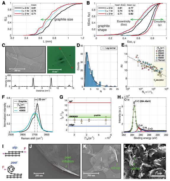
Figure 4.
Shear exfoliation process and graphene morphology and quality. All of the data are presented for the Taylor–Couette flow device. (A) Cumulative size distribution of graphite flakes during processing. (B) Cumulative eccentricity ( , a > b) and circularity (
 ) distributions of graphite flakes during processing. (C) A folded monolayer graphene sheet, including diffraction pattern and peak intensities. (D) Distribution of number of layers using AFM. (E) Average number of layers in solution over exfoliation time, measured using ex situ UV–vis–nIR spectroscopy. (F) 2D peaks and (G) ID/ID' from Raman spectroscopy. (H) High resolution XPS core level spectra for C1s of exfoliated graphene. (I) Illustration of slip and peel exfoliation routes. (J) TEM showing peel initiation site. (K) TEM and (L) SEM showing instances of complete roll-up of liquid exfoliated nanosheets. Experimental conditions: Ci = 10 g l−1,
  s−1 (A) and (B),
  s−1 (C, D, H, J, K, L).
Download figure:
Standard image High-resolution imageAt the nanosheet level, graphene dispersions were analyzed using transmission electron microscopy (TEM), atomic force microscopy (AFM), and scanning electron microscopy (SEM) to study morphology, and using x-ray photoelectron spectroscopy (XPS) and Raman spectroscopy to assess material quality and degree of defects, shown in figures 4(C) and (K). We observed monolayer sheets (figure 4(C)) and log-normal sheet thickness and length distributions (figure 4(D) and section S2), a common feature of exfoliation processes [31]. The long tail in the distribution of number of layers in figure 4(D) leads to some occurrences of graphitic material (N > 10), however, the majority of flakes were found to be within the range classified as FLG (N < 10). Indeed, in figure 4(D) the contribution of monolayer, bilayer and tri-layer nanosheets were found to be 14%, 21% and 16%, respectively. Interestingly, the smallest particles observed were ~10 nm in length, suggesting that the graphite erosion process produces little or no carbon dots. The absence of nanosheet breakage at this scale (~1 nm) is connected to the energy-containing flow structures. The vast majority of energy dissipation ( 90%) occurs at length scales an order of magnitude above the Kolmogorov length (
 ), hence there is insufficient energy budget for reducing the particle length below this. We tracked the change in average number of layers during exfoliation, shown in figure 4(E). Minor sensitivity to strain rate is observed, a result which is controlled by the post-production centrifugation protocol (Materials and methods). This finding was supported by measurements of 2D-bands from Raman spectra in figure 4(F), also used to independently calculate layer number from the 2D peak shape in figure 4(E) using the metric provided by Backes et al [11]. Maintaining the same centrifugation protocol throughout, however, we find sensitivity to exfoliation exposure time, revealing the multiple scales of shear exfoliation. Stress fields erode the precursor at the microscale as shown in figures 4(A) and (B) and 1(C), while simultaneously separating graphene layers from already exfoliated material at the nanoscale (figure 4(E)). Average layer number reduces even when production saturates, as the dispersion of FLG continues to exfoliate. This finding suggests the rate-controlling processes for concentration and selectivity span the entire energy-containing range, from the largest turbulent motions in the fluid gap (
 ) down to the smallest, where nanosheet size is comparable to the Kolmogorov length (
 ). Notably, this demonstrates that tunable average layer number via exfoliation time is possible, without the need for additional secondary liquid processing techniques.
We confirm the quality of graphene is unaltered by strain rate level, with the ratio of D and D' peak intensities ID/ID '
 in figure 4(G). Considering this graphite precursor contains vacancy defects prior to exfoliation, the findings for exfoliated graphene are characteristic of edge defect contributions. The ID/IG ranged from 0.195 to 0.3 with no observable dependency on strain rate (figure S2(A)). This range of ID/IG is similar to that found in other graphene exfoliation studies and attributed to the defect-induced scattering created from nanosheet edges [11]. Combined with a low intensity, narrow D-band obtained from Raman spectroscopy (section S2), XPS measurements in figure 4(H) confirm that graphene is produced without oxidation. Instead, the smaller peaks at binding energies greater than the C–C peak can be explained by residual NMP [4, 14]. NMP atomic populations for the ratio C–H:C–N:C=O are expected to be 3:1:1, and measurements using XPS closely follow this at 3:0.93:0.8 (using a Shirley type background) and 3:1.1:1.57 (using a Tougaard background).
Finally, we found evidence of both slip and peel exfoliation routes, illustrated in figure 4(I), from TEM observations in figures 4(J) and (K) and wider field SEM observations in figure 4(L). The shear exfoliation process can fold, partially roll, or completely roll-up graphene nanosheets into scrolls with an interlayer spacing of 0.34 nm (section S2). Peeling was recently shown using molecular dynamics to require less work to delaminate [24]. Our experimental observations are non-unique to these hydrodynamic conditions, as we observed this peeling effect with Taylor–Couette flows, spinning disc flows (section S2), and elsewhere in the literature [13].
2.3. Real-time monitoring of graphite exfoliation
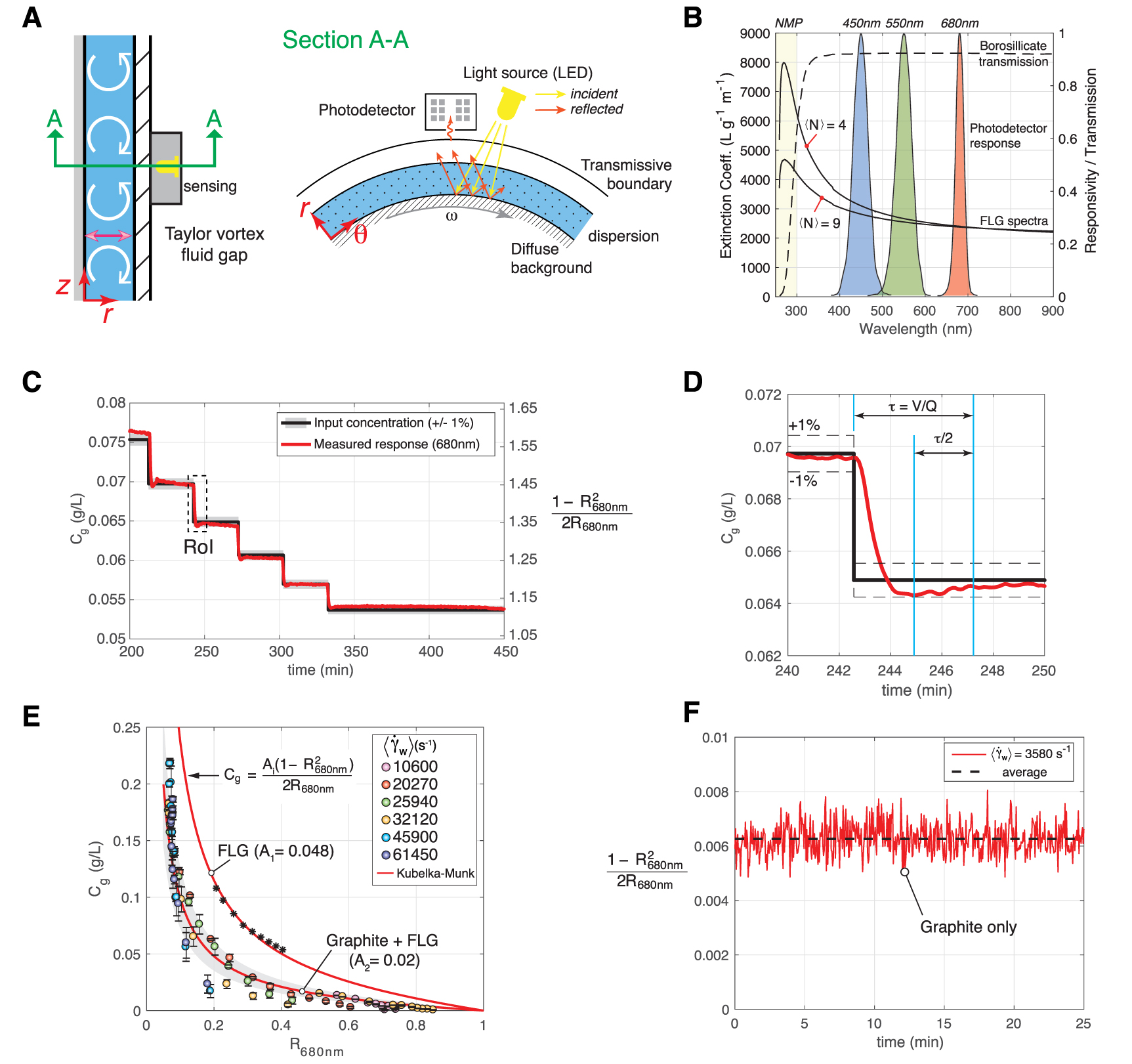
Following the complete analysis on the hydrodynamics of exfoliation and the nanomaterial produced (via contemporary ex situ characterization techniques), we devised a low-cost and scalable in situ technique to monitor graphene production in real-time. We continued with the Taylor–Couette system as the platform to demonstrate the operating principle and assess the suitability for real-time monitoring of graphene production during liquid exfoliation. The approach implements a variation of transmission-reflectance spectroscopy, traditionally considered for static solids/powders and coatings [32]. Using a simple sensing arrangement shown in figure 5(A), we actively measured the optical properties of dynamic, liquid dispersions of nanomaterials during processing without the need for resource-demanding post-processing steps (e.g. centrifugation) or expensive optical components associated with contemporary ex situ spectroscopy methods.
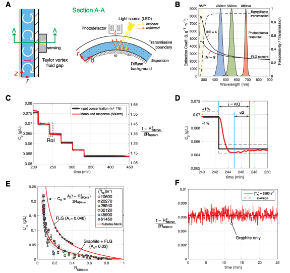
Figure 5.
Real-time monitoring of liquid exfoliation. (A) Device set up for transmission-reflectance spectroscopy of fluids in motion. Light source and detector are positioned external to the Taylor vortex fluid gap. Section A-A illustrates the light path and interactions across boundaries (see movie S4 for operation also). (B) Normalized multispectral photodetector sensitivity (centered on 450 nm, 550 nm, 680 nm), borosilicate window transmittance, and graphene absorbance spectra (from ex situ UV–vis–nIR transmission spectroscopy). (C) Comparison of graphene concentration profiles using Kubelka–Munk theory to transform reflectance measurements at 680 nm into concentration, where  . (D) Enlarged view of the 240–250 min time interval in panel (C) illustrating the system response to step-changes in concentration (RoI from C). (E) Reflectance-concentration profiles for graphene dispersions (FLG) and during the production of graphene from graphite/NMP mixtures (Graphite + FLG, Ci = 10 g l−1 and 1 g l−1). (F) Measurements for a graphite/NMP dispersion while operating below the strain rate required to exfoliate graphene nanosheets (Ci = 10 g l−1).
Download figure:
Standard image High-resolution imageThe sensing platform was located external to the exfoliation process and non-intrusive (movie S4). A light emitting diode (LED) with a broad spectral distribution from 400 to 800 nm provided incident light. This incident light passed through a stationary outer transmissive boundary (borosilicate glass, optical characteristics in figure 5(B)) and the Taylor vortex fluid gap containing the liquid dispersion. It reached a moving background (rotating cylinder) where the light diffusely reflected off the stainless-steel surface. Reflected light from this rotating diffuse background returned through the liquid dispersion and transmissive boundary, doubling the absorbance path length ( ), before reaching a multispectral photodetector comprising a fixed aperture and photodiode arrays sensitive from visible to near-infrared wavelengths (Materials and methods). Optical characteristics of the background and transmissive boundary remained constant; crucially, however, light absorbance and scattering in the interstitial fluid gap can change during 2D material processing.
Gaussian filters provided spectral responses with full width at half maximum (FWHM) of 40 nm (centered on 450 nm, 550 nm) and 20 nm (centered on 680 nm), respectively. These three spectral responses are shown in figure 5(B) and were chosen to: (a) enable measurement of FLG concentration in the near-infrared (680 nm) where the extinction spectra are unaffected by nanosheet dimensions; and (b) capture changes in the shape of FLG spectra in the visible region (450 nm, 550 nm) that are associated with average number of atomic layers in a liquid dispersion [11]. Although changes in spectra are more distinctive towards the  –
– * peak (
 nm), we limited sensing to a shortest wavelength centered on 450 nm due to optical constraints of the exfoliation system. Borosilicate glass transmission reduces significantly below 350 nm. The
  –
– * peak for graphene occurs in a wavelength region where NMP and other solvents are highly absorbent, potentially masking the spectral peak. Finally, the LED light source has a normalized spectral power with maxima closely aligned to the photodetector responses centered on 450 nm and 550 nm, respectively.
Measurement sensitivity to nanomaterial concentration was investigated first by introducing a graphene/NMP dispersion with a known initial concentration (0.075 g l−1) into the Taylor–Couette device and monitoring reflectance during operation at  . We note that all reflectance measurements (
 ) discussed throughout relate to the reflectance of the diffuse background surface. This reflectance signal is altered by the absorption of incident and reflected light passing through the fluid gap (figure 5(A)). Multispectral reflectance data (a.u.) were acquired simultaneously at 3 s intervals, with an integration time of 280 ms (movie S4). We then added NMP (100 ml) to the graphene dispersion every 30 min and tracked the response as shown in figure 5(C). We found that the graphene concentration correlates with Kubelka–Munk theory
  , where K and S are absorption and scattering coefficients; the correlation predictions remain accurate to within ±1% over hours of processing. While
  was obtained for FLG under exfoliation conditions (88% of Z1 is above
  s−1), we can assume the measured changes to be entirely associated with graphene concentration (
 ), as absorption and scattering coefficients in the near-infrared are independent of nanosheet dimensions. Over a shorter time interval (
 min), the system response to step changes in concentration were revealed in figure 5(D), with a time constant in agreement with first-order prediction (
 , where V and Q are process volume and flow rate, respectively). Hence, the technique is sensitive to solution concentration and has potential to monitor, in real-time, the kinetics of nanosheet dispersion processes such as ink and composite formulation.
Extraction of graphene concentration during exfoliation of a graphite precursor was also demonstrated by comparing ex situ concentration measurements with in situ transmission-reflectance data across all hydrodynamic conditions studied in the present work. In figure 5(E), we observe the same correlation with reflectance,  for the heterogeneous system (curve fitting R2 = 0.93), and a lower constant (Ai), that results from increased absorption by the additional graphitic material in the system. Remarkably, this reduced the reflectance (
 ) by only 58%, despite FLG consisting of
  of the total graphite mass.
Measurements for a graphite dispersion and sub-critical exfoliation strain rates are shown in figure 5(F). A low magnitude output over time is observed when compared to the data for graphene only dispersions in figure 5(C). A constant value with small temporal variations exist due to graphite flakes passing the detector, indicating little or no exfoliation occurs. Using the correlation for Graphite + FLG dispersions in figure 5(E), a concentration of ~1 x 10⁻⁴ g l−1 is predicted from the time average data. This is also the lower limit of FLG detection for the measurements presented. The upper limit of FLG detection for our experimental setup was ~0.25 g l−1. Near this level of concentration (figure 5(E)), the reflectance data began to saturate with low levels of light entering the detector. Beyond this work, this limit could be addressed using a different arrangement with a smaller path length for the light to travel (e.g. a gap width < 2 mm), analogous to changing cuvette designs in traditional ex situ UV–vis–nIR spectroscopy.
Owing to a unique electronic structure, graphene absorbs a significant fraction of incident light (2.3%), and this increases linearly with each layer number up to  [33]. Hence, FLG with five layers can absorb over 20% of the light (>10% incident, >10% reflected). Considering the characteristic log-normal distribution in liquid exfoliation shown in figure 4(D) previously, the number density of these few-layer sheets is high. By contrast, the number density of large graphite particles is low, graphitic particle surfaces can be reflective (movie S1), and incident/reflected radiation predominantly penetrates the fluid gap where well-dispersed nanosheets absorb light. Additionally, while the exfoliation process has been shown to reduce graphite size over time in figures 4(A) and (B), particles remain large enough for
  to be independent of size with
  , where
  is the molar extinction coefficient,
  is the molar concentration, and
  is the particle diameter [32].
Large nanographite flakes exfoliated from the graphite precursor can also interact with the incident/reflected light. The scattering behavior of high-aspect-ratio nanoparticles can vary with particle size, and occurs predominantly in a transitional region between Rayleigh and van der Hulst approximation limits [34]. To explore the impact scattering may have on the measurement technique, we applied the empirical correlation proposed by Harvey et al [34] to graphene in NMP. Plotting the small and large sheet limits for a broad range of particle lengths, we find that scattering will have a weak effect on the measurements (figure S16). At large particle sizes,  μm, the scattering intensity reduces, following the large sheet limit (van der Hulst). This behaviour works favorably for the proposed measurement technique, with diminishing scattering effects from large exfoliated particles that are present in solution.
These observations suggest changes in  during exfoliation are primarily due to the absorption of light by nanosheets in dispersion. We confirm this in figures 5(E) and 6(A), as the technique captures nanosheet concentration from these heterogeneous mixtures when graphene is being produced (
 ) and when graphene production saturates (
 ). This capability to experimentally observe graphene concentration within dynamic, heterogeneous dispersions (solvent, graphite and graphene) is essential to enabling real-time monitoring of 2D material production and quality control at large production scales.
2.4. Applications in production, material selectivity and solvent design
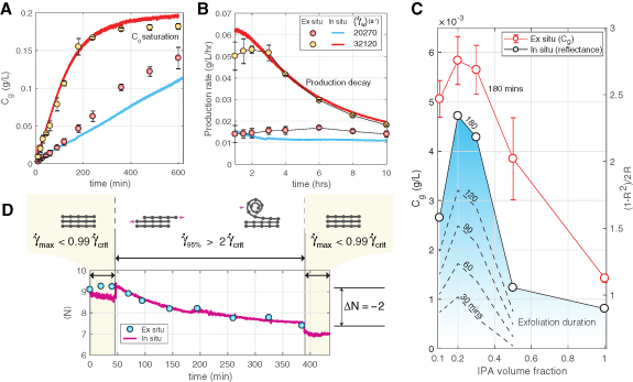
Applications central to the advancement of 2D material production were selected to examine the flexibility of the transmission–reflectance spectroscopy method for process monitoring. Firstly, we examined real-time, quantitative monitoring of graphene production during shear-assisted liquid exfoliation in NMP. Using the Taylor–Couette system, linear and non-linear concentration profiles shown in figure 6(A) were generated. We repeated the same hydrodynamic conditions, incorporating in situ monitoring, and measured graphene concentration in real-time as exfoliation proceeded (using a predetermined Kubelka–Munk relationship from figure 5(E)). Both concentration-time profiles are closely captured (RMSE = 15.6% with the RMS-uncertainty = 13.3% for ex situ measurements), including the transition to graphene saturation. Expressing these measurements in the form of production rate ( ) in figure 6(B) shows the potential to optimize the process for maximum output and observe issues detrimental to efficiency in real-time, such as production rate decay.
Figure 6.
Applications of real-time monitoring in graphene production. (A) Detection of graphene concentration profiles. (B) Detection of production rate performance and fall-off. (C) Solvent design and optimization. Measuring graphene concentration profiles for non-toxic H2O/IPA cosolvents,  s−1. (D) Controlling material selectivity on the fly. Exfoliation is activated from approximately 50 to 400 min. Outside of these times, the strain rate is below what is necessary to produce nanosheets. This plot demonstrates simultaneously reducing and measuring the average number of atomic layers under different strain rate conditions. (A) and (B) use the same figure legend. Experimental conditions: (A–C) were performed on graphite/solvent mixtures with Ci = 10 g l−1. (D) was performed on FLG dispersion with initial
  and Cg = 0.054 g l−1.
Download figure:
Standard image High-resolution image
A second application considered was optimization of environmentally benign solvents. The highest performance solvents for liquid exfoliation and dispersion are generally toxic (e.g. NMP), with high boiling points also limiting practical uses [15]. Previous research on carbon nanotubes and graphene have guided solvent and aqueous-surfactant strategies and relied on concentration measurements to assess performance and suitability [35, 36]. Given the overwhelming need for sustainable synthesis, green solvent design and optimization for high performance is necessary to remove the dependence on conventional solvents [37]. In figures 6(C), we demonstrate rapid solvent design for maximum graphene production using low-hazard, low-boiling point water/IPA cosolvents. We performed exfoliation experiments at  s−1 and for a 3 h duration with different IPA volume fractions (0.1–1). The resultant graphene concentration was measured post-centrifugation using ex situ transmission UV–vis–nIR spectroscopy. In parallel, we measured reflectance (
 ) during exfoliation using the in situ transmission-reflectance technique. The different solvents investigated have negligible effect on the absorbance properties in the visible-nIR region. Using our observations that
  , we detected the optimum IPA volume fraction for the cosolvent at 0.2. This corresponded to a measured surface tension of 33 mN m−1, which is in a region where graphene dispersibility is improved [38]. As well as providing instantaneous production information, a main advantage of the in situ technique is the time saved on post-exfoliation nanomaterial separation. Here, the optimal solvent was observed in a fraction of the time taken with ex situ techniques. The latter required taking a sample, leaving overnight to sediment, performing centrifugation and then UV–vis–nIR spectroscopy (Materials and methods). The minimum time to obtain results for one solvent test was 15 h, with the five tests to determine the optimal solvent mixture taking a total
  75 h. Using this in situ approach, we observed the optimal solvent after processing the five different mixtures for 30 min each (total time = 2.5 h). This would allow 30 solvent trials to be performed in the time it takes for one using traditional characterization approaches.
Finally, we explored multispectral functionality to monitor and control the average number of atomic layers of graphene in real-time. We found that the ratio of reflectance intensities,  , describes the average number of atomic layers in FLG dispersions (section S7), analogous to contemporary ex situ transmission spectroscopy observations using extinction intensity ratios in reciprocal form [11]. As with transmission spectroscopy, the method was insensitive for heterogeneous dispersions containing graphite. In figures 6(D), we examined a graphene/NMP dispersion with an initial number of layers
  . Using our findings on the hydrodynamics of shear exfoliation (section 2.1), we varied the exfoliation conditions with time, by altering the stress fields from no exfoliation (
 ) to the promotion of exfoliation, where 95% of the local strain rate distribution in the Taylor vortex region was above
  . We controlled the reduction of average layer number to
  , and maintained this by returning to the initial hydrodynamic state without exfoliation (
 ). An adjustment of
  was observed when rotational speed was changed at
  min and
  min. This indicates there may be process-specific considerations to take into account when using this in situ multispectral technique. Overall, however, we demonstrate the tuning of material selectivity in real-time and provide an opportunity to tailor dispersions on the fly for individual applications.
3. Conclusions
In summary, insights into the hydrodynamics of liquid exfoliation have been uncovered across all exfoliation scales, from precursor to 2D material, and a robust spectroscopic technique was developed to monitor exfoliation processes in real-time. The derived hydrodynamic variables of strain rate ( ) and particle residence time (
 ) are dominant parameters that govern the scaling of production (
 ), once the local strain rate distributions are above the minimum shear rate required to overcome van der Waals bonding. This work reveals that there is a characteristic time associated with the delamination of nanosheets from precursor materials. This dependence highlights that broader considerations are required for production intensification and scale-up, beyond the single objective of maximizing strain rate levels. We show that these can be coupled and competing, making it essential to consider both parameters with similar weighting. This has been arrived at by combining exfoliation experiments, 2D materials characterization, hydrodynamics experiments and numerical simulations on Taylor–Couette and spinning disc systems. Validated DNS and LES have provided high fidelity predictions in laminar and turbulent shear exfoliation flows.
Although the investigation has focused on continuous flow processes, the derived parameters and scaling relationship uncovered in this work are applicable to batch exfoliation systems also. For example, changing the size of the vessel relative to the impeller in shear mixing can influence local strain rates and the time precursor particles spend in high shear regions (close to the impeller) versus the time spent in low shear regions (far away from the impeller as the precursor recirculates). Optimizing vessel size for large-scale production output may then depend on trade-offs between intensification (e.g. maximizing strain rate and residence time) and the process volume (e.g. maximizing the quantity of material produced in each batch). A direct connection between these findings, batch processing methods and other 2D materials would be beneficial. Together with the present work, it would support the development of a framework to allow practitioners to investigate and design 2D material production and dispersion processes in a virtual environment (e.g. using computational fluid dynamics). This could accelerate the translation of lab processes to industrial scale, and facilitate energy and environmental considerations before moving to physical scale-up activities.
High speed optical measurements of graphite during shear exfoliation conditions revealed the motion and physical material removal process on a particle scale. A graphite erosion process proceeds concurrently with exfoliation of graphene nanosheets and nanoplatelets already in dispersion. This was determined by characterizing the precursor and few-layer materials across concentration growth and saturation regimes. Rate-controlling processes in turbulent exfoliation have been found to span the entire energy-containing range. Small particles such as carbon dots were absent, suggesting the energy budget approaching the Kolmogorov scale becomes insufficient for particle breakage. We observed nanosheet edge folding and roll-up that indicate peel exfoliation is present, and also showed that these structures are non-unique among different shear exfoliation methods. This presents an opportunity for future research into deliberate tailoring of materials and their morphology for applications.
Combining hydrodynamic predictions of strain rate distributions with real-time monitoring of shear exfoliation, we demonstrated nanosheet layer control on-the-fly by applying known stress fields to FLG dispersions. This low-cost multispectral transmission-reflectance spectroscopy approach ( $5 USD) was found to be capable of measuring 2D material concentration and production rate in the presence of the precursor material. This was shown to facilitate high-throughput quality control, process optimization and intensification, and green solvent assessment. The solution avoids time-consuming post-production nanomaterial preparation, ex situ measurements and makes real-time characterization of 2D materials accessible to individuals, labs and industry. Real-time monitoring has been tested for graphene dispersions synthesized from initial graphite concentrations up to ~10 g l−1. Although this range covers most previous studies on liquid exfoliation, an assessment for higher initial graphite concentrations (e.g. ~100 g l−1) would also be beneficial. The realization of the proposed approach has been simplified by the optical characteristics of graphene. Further investigations are necessary to extend this to other 2D materials where light scattering effects can dominate. Despite this, it could easily be extended to other layered materials by selecting photodetector spectral bands coinciding with features from optical spectra that are sensitive to concentration and nanosheet size.
4. Materials and methods
4.1. Experimental methods
Exfoliation experiments were prepared by introducing graphite flakes (Sigma Aldrich, part no. 332461) into a liquid solvent (NMP, or H2O/IPA cosolvents) at a typical concentration of Ci= 10 g l−1 or lower. The process volume for both Taylor–Couette and spinning disc devices was 1.5 l. The graphite/NMP mixture was circulated in a closed loop from a reservoir to the device using a peristaltic pump operating at a volumetric flow rate of 325 ml min−1 (Taylor–Couette) and 360 ml min−1 (spinning disc). A description of the key dimensions for each exfoliation device is included in section S1 (supplementary information).
4.2. Material characterization
Optical microscopy measurements were performed (figure 1(C)), and size distributions were quantified using a laser diffraction particle size analyzer (Malvern Mastersizer 2000). For the size distribution measurements, sodium dodecyl sulfate (SDS, Sigma Aldrich) was dispersed in de-ionized water up to the CMC = 8.2 mM, creating a solution to prevent particle aggregation. Graphite was added to this SDS/H2O mixture and circulated around the laser diffraction particle analyzer. The as-received graphite precursor (specified as +100 mesh) has a log-normal distribution, with a minimum size of 150 µm and mode of 478 µm (figure S1). This was used for the Taylor–Couette exfoliation experiments. A pre-process was necessary for the spinning disc device, owing to the thin films produced (typ. <500 µm). Particle size was decreased to a mode of 85 µm by ball milling the precursor (planetary ball mill, processed for 1 h at 180 rpm followed by 8 h at 225 rpm using three grinding balls).
Samples were taken during exfoliation experiments to measure graphene concentration with process time. A 20 ml volume was pipetted from the device and allowed to settle overnight (12 h). 90% of the supernatant (18 ml) was centrifuged at 1500 rpm for 2 h (RCFmax = 247 g). From the centrifuged product, 77% of the supernatant was then pipetted. This contained a size distribution of graphene and FLG sheets, and was the product used to perform other ex situ characterization techniques (e.g. Raman, AFM, TEM, SEM). This protocol was designed to obtain an average layer number of <10 towards the middle-to-end time of the exfoliation experiments (e.g. No > 105 in figure 4(E)). For 80% of the total processing time, the average layer number was below ten. Graphene concentration was obtained by passing 500 ml of centrifuged product through a PTFE filter (0.45 µm) and measuring the filtered mass. The filter membrane was dried in a vacuum oven at 50 °C and  mbar over 4 days for solvent removal. Evidence of residual solvent was found using XPS measurements (figure 4(H)), however, it had negligible effect on the mass measurements. UV–vis–nIR spectroscopic measurements were performed on the liquid dispersions (Perkin Elmer Lambda 35), and the extinction coefficient was found to be 2322 l g−
1 m−
1 at 750 nm, similar to that found elsewhere [4]. Using the Lambert-Beer relationship (E/l=
mbar over 4 days for solvent removal. Evidence of residual solvent was found using XPS measurements (figure 4(H)), however, it had negligible effect on the mass measurements. UV–vis–nIR spectroscopic measurements were performed on the liquid dispersions (Perkin Elmer Lambda 35), and the extinction coefficient was found to be 2322 l g−
1 m−
1 at 750 nm, similar to that found elsewhere [4]. Using the Lambert-Beer relationship (E/l=  Cg, where E is the measured extinction, l is the cuvette cell length, is the extinction coefficient), graphene concentration data (Cg) were directly measured from the centrifuged liquid dispersions using UV–vis–nIR spectroscopy. The standard deviation across the entire range of concentration measurements (Cg ~ 10−4–10−1 g l−1) is presented in figure 5(E). The RMS uncertainty in concentration data was 13.3%, with a maximum of 33%. Largest uncertainties occurred at early production times (~10 min) when there was a high rate of change to low concentration values.
The quality of exfoliated graphene was investigated with Raman spectroscopy (Bruker, Senterra II). Defects, characterized by ID/ID', were measured across a range of strain rates to assess the impact of hydrodynamics on material quality (figure 4 (G)). Typical normalized spectra are shown in section S2 for the graphite precursor and graphene produced at two different strain rates. Measurements were achieved on vacuum filtered samples with PTFE membranes, using 50× magnification, a 532 nm laser, 6.25 mW intensity and a 2 s integration time. This laser power was chosen to produce a strong Raman signal without introducing degradation to material quality. Although spectra can be sensitive to temperature dependencies, previous work has shown that this laser power is suitable for FLG characterization with no significant D band contributions and constant G mode response to changes in laser power from 1 to 9.5 mW [39]. Ten locations were measured for each sample, with five co-additions each. The spectra were post-processed using Matlab to perform background subtraction, normalize spectra to the G peak and conduct peak-fitting. Background subtraction was performed using a method based on minimizing a non-quadratic cost function for a low-order polynomial fit [40]. Lorentzian peak-fitting was performed to quantify ID', ID, and I2D' (section S2).
XPS was used to assess oxidation of the material in figure 4(H) (Thermo Scientific K-Alpha). Vacuum filtered graphene was carefully removed from the membrane and mounted to the XPS sample holder using conductive carbon tape. X-ray gun power was set to 72 W (6 mA and 12 kV). All high-resolution spectra (C1s and O1s) were acquired using 20 eV pass energy and 0.1 eV step size with 50 scans. Data was analyzed using Thermo Avantage software (ThermoFisher Scientific). A recommended 'Smart' background was used which is based on the Shirley background. The data was also processed using a Tougaard background. The Powell peak fitting algorithm was used and spectra were shifted to align the peak for adventitious carbon C−C at 284.7 eV.
The thickness and shape of graphene nanosheets were measured using Atomic Force Microscopy (Bruker Dimension Icon). Measurements were performed in peak force tapping mode with ScanAsyst at resolution of 256 × 256 and line rate of 1.5 Hz. The setpoint was set around 150 pN. The cantilever used was ScanAsyst Air with spring constant of 0.4 N m−1. Dispersions were diluted to an optical extinction of 0.15 at 750 nm and drop cast onto a freshly cleaved mica sheet (25 mm × 25 mm) at 10 μl per 5 mm2. Drop casting was performed on mica which was preheated to ≈ 220 °C, rapidly boiling off NMP and minimizing re-aggregation of nanosheets. Microscopy images obtained with TEM are commonly used for nanosheet size measurements, owing to the higher spatial resolution over AFM. A disadvantage of this approach is that size and thickness measurements are obtained from two different sets of samples. We quantitatively assessed the limitation of AFM images for measuring the size and shape characteristics of nanosheets (section S2). We developed an object detection code in Matlab, based on Otsu's method [41], to obtain object properties. Restricting the maximum uncertainty to <20%, we found the measurement limit occurs when the object area and length are below 10 px2 and 3 px, respectively. When measuring the size of nanosheets, we ignored objects below these thresholds. Following this, we assessed the sensitivity of measurements to AFM resolution. First, a wide field of view (FoV) image was acquired with a resolution of 0.05 px nm−1 (section S2). Two different nanosheets were isolated and scanned at several times the resolution to obtain images that provide similar detail as the TEM technique. The object detection method was then applied to both high- and low-resolution measurements and geometric details on each nanosheet were compared. The maximum measurement errors were found to be 3.4% (max length), 6.3% (min length), 8% (area), 11.6% (height), 6.6% (perimeter), and 3.1% (eccentricity). These were considered acceptable differences, and analyses on size and thickness statistics (e.g. figure 4(D)) were performed on wide FoV (5 μm × 5 μm) AFM measurements obtained at 0.05 px nm−1 resolution. Multiple AFM measurements were recorded and analyzed to obtain statistical information from 200 nanosheets. We also note that the use of semi-automated image analysis was recently shown to be an effective approach for the statistical analysis of graphene nanosheets measured using AFM [42]. Height data was converted to atomic layer number by applying the step height analysis procedure. An apparent layer thickness of 1.7 nm was measured and is similar to that found elsewhere for liquid-exfoliated nanosheets. Finally, we examined the relationship between UV–vis–nIR spectroscopic metrics 550nm/325nm and AFM measurements of average layer number, finding it to be in agreement with the literature [11]. This metric was used to calculate average layer number across the large processing space in figure 4(E).
Nanosheet morphology was also investigated using the TEM technique (JEOL 2100plus, 200kV, Magnification range 4000× to 100 000×). Samples were prepared on holey carbon film 300 mesh copper support grids. Three drops were deposited on the carbon grid using dispersions with an optical extinction of 0.15 at 750 nm. To remove residual solvent, samples were dried over 3 days at 120 °C in a vacuum oven before performing measurements. Electron diffraction patterns were also measured (figure 4(C)). To obtain a larger FoV of the processed material (figure 4(L)), SEM measurements were performed (Zeiss Auriga, 5kV). Graphene powder from filter membranes was extracted with a carbon black tape, blown with compressed air to remove excess powder, and placed on the SEM sample holder. Measurements aligned with TEM observations that both slip and peel routes frequently occur in shear-assisted liquid exfoliation processes.
Finally, measurements of surface tension for each H2O/IPA cosolvent examined (figure 6(C)) were performed using a pendant drop analysis method (Kruss).
4.3. Graphite precursor tracking
The graphite precursor was tracked across multiple spatio-temporal scales (from μm and μs to mm and hours) during shear-assisted exfoliation. This was achieved on the Taylor–Couette device by providing optical access to the exfoliation region (Z1, figure 1(B)). The stationary outer cylinder was constructed from borosilicate glass, providing a complete 360° view of the fluid motion during exfoliation (movie S1).
Images of individual graphite particles under exfoliation conditions were obtained using a high-speed camera (Olympus i-SPEED 3) with 60 mm or 105 mm lens (Nikon AF-S Nikkor, f/2.8). Lighting was provided using two halogen lamps mounted either side of the camera (section S3). Images were acquired at different frame rates ranging 2000–10 000 fps depending on the flow speed and FoV under investigation. Exposure time was adjusted in the range 30−100 μs to balance image intensity and avoid particle blurring/streaking. Quantitative information was obtained by calibrating the images using a checkered grid with known spacing placed inside the device prior to performing exfoliation runs (section S3).
Particle image velocimetry was performed on images to extract the graphite velocity field in the axial-azimuthal direction (figure 1(C)). An open source two-pass FFT window deformation approach developed in Matlab [43] was used to calculate velocity fields from image pairs with a Δt based on the camera frame rate. Each image pair was divided into interrogation regions of 64 × 64 pixels and 32 × 32 pixels for first and final passes (both with 50% overlap). This resulted in a velocity vector every 800 μm. A sufficient number of samples (>500 image pairs) were considered to ensure ensemble averages were statistically representative of the time-averaged particle motion [44]. Particle tracking velocimetry was also performed to extract the paths of individual graphite particles (figure 1(C), movies S1 and S2). An open source method developed in Python was used to perform feature finding in images with sub-pixel precision and then link time information to obtain feature trajectories [45]. A total of 2500 frames were analyzed, ignoring agglomerated/grouped particles to ensure that tracking was performed on individual graphite flakes. We selected minimum particle displacements of 3 px and filtered the trajectories to particles who were present for 50 consecutive frames or more. The uncertainty in particle velocity was estimated to be less than 3% [44].
The rheoscopic effect was monitored over the complete exfoliation process using an 8 MP Sony IMX219 camera module connected to a Raspberry Pi which controlled acquisition. To quantify the band numbers in the images that result from the Taylor vortex instability, a FFT was applied in the image processing. First, the intensity profile in each column is extracted from the image. Then, the FFT is applied to each column and a frequency profile is obtained. The band number with the dominant signal strength is chosen to represent how many bands are found in a particular column. Finally, the mode of all band numbers from all columns is defined as the number of bands in the picture. Fluctuations in band number over 10 h processing were consistently centered about a mean of 11 bands, typically varying by ±1.
The graphite exfoliation process was investigated by taking high-speed images at three different exfoliation times (0, 1 and 2 h), and analyzing the particle size and shape (figures 4(A) and (B)). The same experimental configuration was used to acquire and calibrate the images as described above for particle image/tracking velocimetry. A minimum of 500 individual particles were manually selected, avoiding particle groups. Particle size and shape was then extracted using the same object detection approach described for nanosheet characterization above. This resulted in an estimated uncertainty of less than 4%.
4.4. Simulation of exfoliation methods
Simulations were performed using the open source computational fluid dynamics code, OpenFOAM on High Performance Computing facilities. The hydrodynamics of the Taylor–Couette process were modeled using a LES method with Wall Adapting Local Eddy-Viscosity sub-grid scale approach [46] to model turbulence below the Taylor microscale. A 360° section of the exfoliation region (Z1, figure 1) was modeled using periodic boundary conditions in the axial direction. Boundary conditions at inner ( ) and outer (
 ) cylinder surfaces were no slip. The length of the domain in the z-direction was
  , where
  is the fluid gap width. The grid comprised 10 M hexahedral cells with a near wall
  , where
  is the shear velocity,
  is the distance normal to the cylinder surface and
  is kinematic viscosity. The thin film flows over the Spinning disc were modeled using DNS and a geometric volume-of-fluid (VoF) approach to capture the interface between the liquid film and gas [47]. A 50° sector of the exfoliation region (Z1, figure 2) was modeled using rotationally periodic boundary conditions, no slip for the disc surface (
 ), a constant nozzle inlet velocity and zero gradient for the outlet at the disc periphery (
 ) and at the gas boundary (
 ). The grid comprised 70 M hexahedral cells with a minimum local grid resolution in the liquid film of ten cells. The incompressible Navier–Stokes equations were solved using second-order discretization schemes. Newtonian fluids were modeled, reflecting the solvents used in the experiments (NMP, IPA, H2O). The graphite phase was neglected based on testing at very low volume fractions typical of exfoliation studies in the literature. The governing equations for both numerical approaches (DNS, LES) are included in section S4.
Local strain rate distributions, histograms and averaged statistics were post-processed from the DNS and LES solution data using ParaView and Matlab (e.g. figure 3, section S5). The simulation methods were validated against the exfoliation experiments in the manuscript and independent data from the literature (section S4).
The LES method was validated against DNS on Taylor–Couette flow within the range of Reynolds numbers investigated for exfoliation (3000 < Re < 13 000) [48, 49]. A comparison between the turbulent structures in the fluid gap, wall shear stress patterns, and local velocity fields showed qualitative agreement. Local quantitative validation was confirmed by comparing the angular momentum and velocity fluctuation profiles in the fluid gap between concentric cylinders. We determined an appropriate model constant,  , that reduced the difference between DNS and experiments to <2% for the angular momentum
  , and <10% for the velocity fluctuations
  . Furthermore, we observed bulk torque differences of 5.4%, where
  is the coefficient of torque for the inner cylinder. Particle image and tracking velocimetry measurements (figure 1(C)) provided an additional confirmation of the validity of our LES predictions. As noted in the main text, the particle track angles agree with the predicted turbulent streaks and streamlines (figures 1(C) and 3 (A), movie S2).
DNS and the interface-capturing VoF approach were validated with experiments from the literature [50] and through qualitative high-speed images on the exfoliation experiment (e.g. figure 2(B) and movie S3). The predicted liquid–gas interface captured the wave evolution observed in experiments, including the transition from 'spiral' to 'horseshoe' waves as inertia increases through an increase of the flow rate and/or the rotational speed of the disc. This was important for accurate predictions of local strain rates, as the interfacial waves have a significant effect (figure 3 (C), sections S4 and S5). A quantitative comparison of film height and wave shape was conducted using experimental [50] and simulation snapshots, where local differences in film height of 20%–30% were observed. Given the transient and stochastic nature of the flow (local film height varied 30% over a 5 ms interval), the accuracy of the numerical method was deemed acceptable.
4.5. Real-time production monitoring
The transmission-reflection spectroscopy sensing platform was assembled using a Luxeon 3014 LED (25.5 lm at 60 mA) as the light source and two six-channel photodetectors with independent optical filters (ams, AS7262 and AS7263). This provided a spectral response spanning visible to nIR wavelengths discretized into 12 bands. Of these 12 bands, three were selected for characterizing FLG and centered on 450 nm (FWHM = 40 nm), 550 nm (FWHM = 40 nm) and 680 nm (FWHM = 20 nm). The sensor and light source were controlled by an Arduino UNO microcontroller with communication over I2C. The Arduino UNO was connected to a PC using USB with baud 115 200 and the sensor readings were recorded using a custom Python script. For real-time measurements on heterogeneous mixtures of graphite and graphene, large graphite particles passing the detector produced fluctuations around the mean reflectance that were <1% (figure 5(F)).
Acknowledgments
The authors acknowledge use of High Performance Computing facilities at Imperial College London (DOI: 10.14469/hpc/2232) and University of Birmingham (BlueBEAR). We are also grateful to Dr Sofia Marchesini and Dr Richard Thorogate for the useful discussions on materials characterization topics.
Funding
This research has received funding from the European Union's Horizon 2020 research and innovation programme under the Marie Sklodowska-Curie Grant Agreement No. 707340, and support from the EPSRC CDT in Advanced Characterisation of Materials (2018 NPIF grant EP/S515085/1).
Author contributions
J S and N U performed the exfoliation experiments in NMP, characterizations and numerical simulations. U F and A L carried out Raman spectroscopy and x-ray photoelectron spectroscopy measurements. S F and S W performed exfoliation experiments and measurements of surface tension for water/IPA cosolvents. H C and J S designed techniques to monitor the rheoscopic behavior of dispersions. J S performed the particle image velocimetry and particle tracking velocimetry experiments. J S designed and carried out the real-time spectroscopy experiments. J S, C P and O K M designed the research and wrote the manuscript.