
Abstract
Magnons dominate the magnetic response of ferromagnetic two-dimensional crystals such as CrI3. Because of the arrangement of Cr spins in a honeycomb lattice, magnons in CrI3 bear a strong resemblance with electrons in graphene. Neutron scattering experiments carried out in bulk CrI3 show the existence of a gap at the Dirac points, conjectured to have a topological nature. We propose a theory for magnons in CrI3 monolayers based on an itinerant fermion picture, with a Hamiltonian derived from first principles. We obtain the magnon dispersion for 2D CrI3 with a gap at the Dirac points with the same Berry curvature in both valleys. For CrI3 ribbons, we find chiral in-gap edge states. Analysis of the magnon wave functions in momentum space confirms their topological nature. Importantly, our approach does not require a spin Hamiltonian, and can be applied to insulating and conducting 2D materials with any type of magnetic order.
Export citation and abstract BibTeX RIS

Original content from this work may be used under the terms of the Creative Commons Attribution 4.0 license. Any further distribution of this work must maintain attribution to the author(s) and the title of the work, journal citation and DOI.
1. Introduction
Magnons are the Goldstone modes associated to the breaking of spin rotational symmetry. Therefore, they are the lowest energy excitations of magnetically ordered systems, and their contribution to thermodynamic properties, such as magnetization and specific heat, has been long acknowledged [1, 2]. More recently, their role in non-local spin current transport through magnetic insulators has been explored experimentally [3] and there are various proposals to use them for information processing in low dissipation spintronics [4]. In this context, the prediction of topological magnons with chiral edge modes [5–7] opens new horizons in the emerging field of topological magnonics [8].
The recent discovery of stand-alone 2D crystals with ferromagnetic order down to the monolayer, such as CrI3 [9], CrGe2Te6 [10], and others [11], brings magnons to the centre of the stage, because of their even more prominent role determining the properties of low dimensional magnets. Actually, in 2D magnets at any finite temperature the number of magnons would completely quench the magnetization, unless magnetic anisotropy or an applied magnetic field breaks spin rotational invariance and opens up a gap at zero momentum [12, 13]. Unlike in 3D magnets, the thermodynamic properties of 2D magnets are dramatically affected by the proliferation of magnons. This is the ultimate reason of the very large dependence of the magnetization on the magnetic field in materials with very small magnetic anisotropy, such as CrGe2Te6 [10].
Magnons in CrI3 attract strong interest and are the subject of some controversy. Experimental probes include inelastic electron tunnelling [14] and Raman spectroscopy [15, 16]. In the case of bulk CrI3, there are also ferromagnetic resonance [17] and inelastic neutron scattering experiments [18]. Only the latter can provide access to the full dispersion curves E(k) = ћω(k). There is a consensus that there are two magnon branches, expected in a honeycomb lattice with two magnetic atoms per unit cell. The lower branch has a finite minimum energy,  , at the zone centre Γ. This energy represents the minimal energy cost to create a magnon and plays thereby a crucial role. Different experiments provide radically different values for
  , ranging from a fraction of a meV to 9 meV [16]. This quantity is related to the crystalline magnetic anisotropy energy that, according both to density functional theory (DFT) calculations [13, 19, 20] and multi-reference methods [21], is in the range of 1 meV.
Inelastic Neutron scattering also shows [18] that, for bulk CrI3, the two branches of the magnon dispersions are separated by a gap. The minimum energy splitting occurs at the K and  points of the magnon Brillouin zone (BZ). As in the case of other excitations in a honeycomb lattice with inversion symmetry, such as electrons and phonons, one could expect a degeneracy of the two branches at the Dirac cone, giving rise to Dirac magnons [22]. Interestingly, second neighbour Dzyaloshinskii–Moriya (DM) interactions are not forbidden by symmetry in the CrI3 honeycomb lattice, and are known to open a topological gap [7], on account of mapping of ferromagnetic magnons with second neighbour DM in the honeycomb lattice into the Haldane Hamiltonian [23]. In contrast with a 'trivial' gap, the opening of a topological gap between the two branches a the Dirac points leads to a finite Berry curvature with the same sign in both valleys that, integrated over the entire BZ, leads to quantized Chern number and a non-vanishing transverse Hall conductivity at zero field [24]. In addition, topological gaps in bulk imply the emergence of in-gap edge states.
The description of magnons in magnetic 2D crystals has been exclusively based in the definition of generalized Heisenberg spin Hamiltonians with various anisotropy terms, such as single ion and XXZ exchange [13], Kitaev [25], DM [7]. Once a given Hamiltonian is defined, the calculation of the spin waves is relatively straightforward, using linear spin wave theory based on Holstein–Primakoff representation of the spin operators [26]. The energy scales associated to these terms can be obtained both from fitting to DFT calculations of magnetic configurations with various spin arrangements [13] as well as to some experiments [18]. However, this method faces two severe limitations. First, the symmetry and range of the interactions that have to be included in the spin Hamiltonian. are not clear a priori. Second, in order to determine N energy constants, N + 1 DFT calculations forcing a ground state with a different magnetic arrangement are necessary and the values so obtained can depend on the ansatz for the Hamiltonian.
The observation of the topological gap in bulk CrI3 does not permit to determine the spin Hamiltonian, because two different types of anisotropic exchange are known to lead to topological magnons in honeycomb ferromagnets with off-plane magnetization. On one side, there are second neighbour DM interactions [7], not forbidden by symmetry in the CrI3 honeycomb lattice. This coupling maps into the Haldane Hamiltonian [23]. On the other hand, first neighbour Kitaev interactions, claimed to be large in CrI3 [17], lead to topological magnons in honeycomb lattices [27, 28].
Here we circumvent this methodological bottleneck and describe magnons directly from an itinerant fermion model derived from first principles calculations. Our approach, that has been extensively used to describe magnons in itinerant magnets [29, 30], is carried out in five steps. First, we compute the electronic structure of the material using DFT, without taking either spin polarization or spin–orbit coupling (SOC) into account. Second, we derive a tight-binding model with s, p, and d shells in Cr and s and p shells in iodine. The electronic bands obtained from this Hamiltonian are identical to those calculated from DFT (see the Methods section for further details). In the third step we include both SOC in Cr and I as well as on-site intra-atomic Coulomb repulsion in the Cr d shell. The resulting model is solved in a self-consistent mean field approximation [30].
In the fourth step, we compute the generalized spin susceptibility tensor  in the random phase approximation (RPA). In the final step we find the poles of the spin susceptibility tensor in the
  space, that define the dispersion relation
  of the magnon modes, where n labels the different modes. More details about the each step are presented in the Methods section.
2. Methods
2.1. Magnons from a Fermionic Hamiltonian
As outlined in the introduction, our approach to calculate the magnon spectrum is carried out in five steps, which we now describe in detail.
Step 1: DFT calculation. We compute the electronic structure of the material using DFT, without taking either spin polarization or spin orbit coupling (SOC) into account. The DFT calculation has been performed with the Quantum Espresso package [31, 32]. We employed the Perdew–Burke–Ernzerhof functional [33] and the ionic potentials were described through the use of projected augmented wave pseudopotentials [34]. The energy cutoff for plane waves was set to 80 Ry. We used a 25 × 25 × 1 Monkhorst–Pack reciprocal space mesh [35].
Step 2: Extraction of the tight-binding Hamiltonian. Now we derive a tight-binding model with s, p, and d shells in Cr and s and p shells in Iodine. The electronic states of the CrI3 monolayer are described by a model Hamiltonian

The first term, describing the tight-binding Hamiltonian for s, p, d orbitals in Cr and s, p orbitals in I is given by
Here,  is the creation operator for an atomic-like orbital µ at site Rl
with spin
is the creation operator for an atomic-like orbital µ at site Rl
with spin  . The hopping matrix
  is extracted by the pseudo atomic orbital (PAO) projection method [36–40]. The method consists in projecting the Hilbert space spanned by the plane waves onto a compact subspace composed of the PAO. These PAO functions are naturally built into the pseudopotential used in the DFT calculation. The bands obtained from this tight-binding model are identical with those obtained from the spin un-polarized DFT calculation. In figure 1(a) we present the band structure of a CrI3 monolayer as obtained from the same ab initio calculation from which we extracted the hopping matrix used our the susceptibility calculations. In the original DFT calculation (details are given above) spin polarization is suppressed and spin-orbit coupling is turned off. The resulting band structure is shown in figure 1(a), together with the bands obtained from the corresponding tight-binding Hamiltonian.
5
is extracted by the pseudo atomic orbital (PAO) projection method [36–40]. The method consists in projecting the Hilbert space spanned by the plane waves onto a compact subspace composed of the PAO. These PAO functions are naturally built into the pseudopotential used in the DFT calculation. The bands obtained from this tight-binding model are identical with those obtained from the spin un-polarized DFT calculation. In figure 1(a) we present the band structure of a CrI3 monolayer as obtained from the same ab initio calculation from which we extracted the hopping matrix used our the susceptibility calculations. In the original DFT calculation (details are given above) spin polarization is suppressed and spin-orbit coupling is turned off. The resulting band structure is shown in figure 1(a), together with the bands obtained from the corresponding tight-binding Hamiltonian.
5
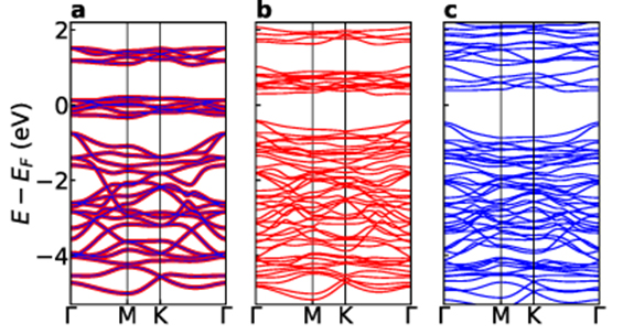
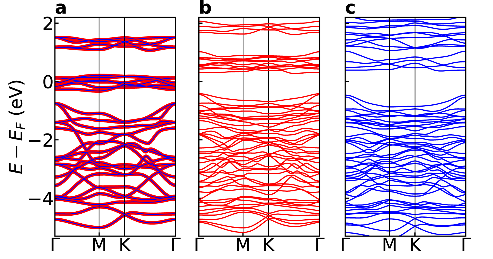
Figure 1. Electronic band structure of a CrI3 monolayer. (a) The results of a DFT calculation without spin polarization or SOC (solid blue lines) superimposed to the results of a tight-binding calculation with a hopping matrix derived from the same DFT calculation. Spin-orbit coupling and spin polarization have been turned off for both calculations. EF stands for Fermi energy. (b) Tight-binding bands after self-consistent mean-field calculation including intra-atomic Coulomb repulsion and spin–orbit coupling. (c) DFT bands with spin polarization and spin–orbit coupling.
Download figure:
Standard image High-resolution imageStep 3: inclusion of Coulomb repulsion and SOC terms. Here we add to the tight-binding Hamiltonian both a screened Coulomb repulsion term,
and a local spin-orbit coupling (SOC) term,
The strength of the spin-orbit coupling is taken from the literature [41],  eV. The screened Coulomb repulsion matrix elements
  are approximated by a single parameter form, which is qualitatively equivalent to taking a spherically symmetric average of the interaction potential [42],

We further assume the repulsion between electrons in s and p orbitals is negligible. Thus, only electrons occupying d orbitals at Cr atoms suffer electron-electron repulsion. The strength of the Coulomb repulsion is chosen as I = 0.7 eV, in order to reproduce the DFT magnetic moment of 3.18  at each Cr site. The total magnetic moment per unit cell is 6
 . The iodine sites acquire a small polarization, opposite to that of the Cr sites. Varying the strength of the Coulomb repulsion in the range 0.5–0.9 eV changes the Cr magnetic moments by more than 12%, while affecting only slightly (less than 2%) the total magnetic moment per unit cell.
The spin-polarized ground-state of the system is obtained within a self-consistent mean-field approximation, in which all three components of the magnetization of each Cr atom within the unit cell are treated as independent variables [30]. For the CrI3 monolayer we find, in agreement with experimental results and DFT calculations, that the ground-state magnetization is perpendicular to the monolayer.
In figure 1(b), we show the tight-binding band structure after the inclusion of Coulomb repulsion (leading to spin polarization) and spin-orbit coupling. For comparison, we show in panel c of figure 1 the bands obtained from a DFT calculation with SOC and spin polarization.
Step 4: Fermionic Spin susceptibility in the RPA. The magnon energies are associated with the poles of the frequency-dependent transverse spin susceptibility,
where

and
The angular brackets  represent a thermal average over the grand-canonical ensemble. The double time Green function
  defined in equation (7) can be interpreted as the propagator for localized spin excitations created by the operator
  . In a system with translation invariance, its reciprocal space counterpart can be readily interpreted as the propagator for magnons with well-defined wave vector.
The transverse spin susceptibility is calculated within a time-dependent mean-field approximation, which is equivalent to summing up all ladder diagrams in the perturbative series for  . These are the same Feynman diagrams that enter into time-dependent DFT. In the presence of SOC, however, the transverse susceptibility becomes coupled to other three susceptibilities, which are related to longitudinal fluctuations of the spin density and fluctuations of the charge density. Thus, it becomes necessary to solve simultaneously the equations of motion for the four susceptibilities [30].
Step 5: Magnon dispersion relation. Finally, we locate the poles of the spin susceptibility tensor in the  space, that define the dispersion relation
  of the magnon modes, where n labels the different modes. For a CrI3 monolayer, which has two magnetic atoms per unit cell, there are two magnon modes. In a general geometry, the number of magnon modes equal the number of magnetic sites. For a system with translation invariance, the number of magnon modes equals the number of magnetic sites in a unit cell.
2.2. Magnon normal modes
In a system lacking periodicity, or with more than one magnetic atom per unit cell, the frequency- (and eventually wave vector-) dependent transverse spin susceptibility can be written as a matrix in atomic site indices,  . There are at least two useful interpretations for this matrix. One originates from its role as a response function in the linear regime, the other is related to its formal similarity to the single-particle Green function of many-body theory.
2.2.1.
 as a linear response function

When interpreted as a linear response function the transverse spin susceptibility yields the change in the transverse component of the spin moment  at site l due to a transverse, circularly polarized external field
  of frequency ω acting on site
  ,
,
We assume the system has N magnon normal modes, where N equals the number of non-equivalent magnetic atoms in the system. Each mode (m) is characterized by complex amplitudes  at the magnetic site l. A general motion of the transverse components of the spin can be written as a linear combination of the normal modes,
Now consider an external field whose frequency and complex amplitudes match exactly those of a normal mode,
In this case, the corresponding change in the transverse spin moment  induced by the field should be proportional to the same normal mode,

Thus,

This shows that the normal modes are the eigenvectors of the susceptibility matrix. In principle, this procedure yields 'normal modes' for any arbitrary frequency of the external field. However, the 'true' normal modes are the ones for which the system responds resonantly. Thus, we can look at the imaginary part of the eigenvalues of  as a function of frequency and associate their peaks with the frequencies of the normal modes.
2.2.2.
as the magnon singe-particle Green function

In order to arrive at this interpretation we can make an analogy with the spin wave theory obtained from the linearized Holstein–Primakoff transformation [43]. There, after linearization, the bosonic operator that represents a spin excitation localized at atomic site l is  . Thus, if we write the definition of the transverse susceptibility replacing
  by bl
and
by bl
and  by
by  , we arrive at a form that is completely analogous to that of the single particle Green function of many-body theory,
Here,  is a thermal average (or a ground state average at T = 0), θ(t) is the Heaviside unit step function. As in the linearized Holstein–Primakoff transformation, the magnons of our RPA theory are independent particles, described by an effective Hamiltonian H composed only of one-body terms. In that case, it is straightforward to show that the Fourier transform of the single-particle Green functions
  are the matrix elements of a matrix
  related to the Hamiltonian matrix by

Thus, the magnon normal modes of the system are the eigenvectors of the susceptibility matrix  where E* are the magnon energies, associated with the peaks of the imaginary part of the eigenvalues of
  .
.
2.3. Berry curvature calculation
The Berry curvature associated with a point in the reciprocal space is a good indicator of possible topological behaviour. Its integral over the whole BZ is called the Chern number, a topological invariant which can be used to classify band structures according to topological properties. In this section we describe a procedure to calculate a numerical approximation to the Berry curvature at an arbitrary point in the reciprocal space. In section 3 we present the Berry curvature of the CrI3 magnons as evidence of their non-trivial topology.
The Berry phase associated to a closed contour C in the momentum space  is given by [44]:
where  is the Berry connection and
  is the Berry curvature.
An efficient way to compute the Berry curvature at a given point  is to compute the Berry phase in a infinitesimal loop in the plane
  [45]. We parametrize the line integral with the variable θ,

Now we note that the argument of the integral has to be purely imaginary, since  . We thus have:

We discretize the integral and the derivative:
We expand this expression:

Now we use the fact that the overlap is close to 1 so that  is a small number. We use the expression log(1 +
  ) ≃ and write:
Now we use  to write:
This expression is convenient for numerical evaluation, because random phases are eliminated, as all states appear twice as conjugated pairs. Therefore, random phases that inevitably occur in the numerical diagonalizations are cancelled.
We now consider an infinitesimal loop of area  formed by 3 points,
  . We now introduce the notation for the overlap

to write the Berry phase in the loop as

Thus, the Berry curvature is obtained as:

3. Results and discussion
The 2D CrI3 magnon dispersion along the high symmetry directions of the BZ are shown in figure 2, calculated both with and without spin orbit coupling, ξI
. As expected for a unit cell with two magnetic atoms, we find two branches of magnons. At the Γ point, spin orbit coupling opens up a gap  , as expected [13]. At the K and
  points, the two magnon branches form Dirac cones when ξI
= 0, but a gap
points, the two magnon branches form Dirac cones when ξI
= 0, but a gap  opens up, whose magnitude is an increasing function of the iodine spin orbit coupling. In order to assess the topological nature of the gap at K and
  points, we first examine the wave functions for the two modes along the
  line. The magnon wave functions can be written as linear combinations of spin flips across the Cr honeycomb lattice, with weights cA
and cB
on the A and B triangular sublattices:
line. The magnon wave functions can be written as linear combinations of spin flips across the Cr honeycomb lattice, with weights cA
and cB
on the A and B triangular sublattices:
where n labels the branch. A distinctive feature of topological quasiparticles in the honeycomb lattice [23, 46] is the braiding in momentum space of the sublattice components. In panels a and b of figure 3 we plot the coefficients  and
and  , obtained from our itinerant fermion model, as
  traces the high symmetry directions of the magnon BZ. As
  goes from K to
  , for a given
  behaves as a spinor that goes from the north to the south pole, with the reverse behaviour for the other branch, exactly as in the Haldane model. We have verified that this pattern is reversed if the off-plane magnetization changes sign.
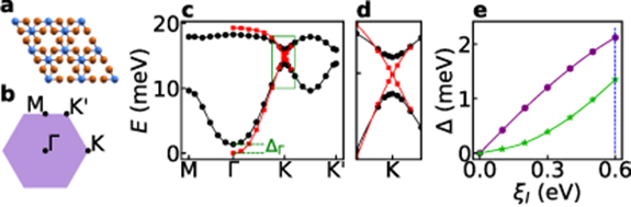
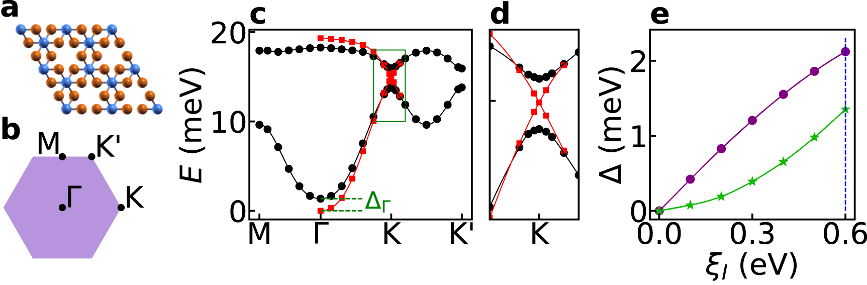
Figure 2. Energy dispersion magnons in CrI3 monolayer. (a) Crystal structure of CrI3 (top view, Cr atoms in blue, I atoms in orange). (b) Brillouin zone, with high symmetry points. (c) Energy dispersion of magnons for 2D CrI3 monolayer, obtained from the poles of the spin susceptibility tensor, computed for a ferromagnetic ground state (black circles). The data for the red squares were obtained from a calculation where the SOC strength at the I atoms has been set to zero. (d) Zoom into the topological gap (the region marked by a green rectangle in panel (c). In the absence of SOC the magnon modes are degenerate at K, as evidenced by the red squares. (e) Size of the topological gap ΔK
(purple circles) and of the anisotropy gap  (green stars) as a function of the SOC strength in the iodine atoms. The blue dashed line marks the actual value for
  used in the calculations of the magnon spectrum. All lines in panels c, d and e are guides to the eye.
Download figure:
Standard image High-resolution image
Figure 3. Analysis of the magnon wave function coefficients (equation (26)) for a CrI3 monolayer. Coefficients cA
and cB
for lower (a) and higher (b) energy branch along the  line in the Brillouin zone. It is apparent that at the Dirac points
  , the spinor is sublattice polarized: the sign of the polarization changes as we change either the branch or the mode, following a braiding pattern, exactly like in the Haldane model. (c) Berry curvature, for both magnon branches, along the
  line in the Brillouin zone. For a given branch, the Berry curvature has the same sign in both valleys, that give the dominant contribution. The sign of the Berry curvature is opposite for both branches. Thus, the integrated Berry curvature is clearly finite, with opposite signs for the two branches.
Download figure:
Standard image High-resolution imageTopological magnons have a finite Berry curvature that leads to non-zero Chern number when integrated over the entire BZ [5–7]. In figure 3(c) we show the Berry curvature along the high symmetry line Γ-K- in the BZ (see the Methods section for calculational details). The Berry curvature of a given mode peaks at the K and
  valleys, with the same sign. Therefore, we expect a non-zero Chern number and hence the existence of in-gap chiral edge modes
6
.
valleys, with the same sign. Therefore, we expect a non-zero Chern number and hence the existence of in-gap chiral edge modes
6
.
Our calculations (figure 2(e)) give strong evidence that the topological gap is driven by the spin orbit coupling of iodine. Thus, the finite Berry curvature has to be produce by inter-atomic exchange mediated by the ligand. A very likely candidate is second neighbour DM interactions, that are known to result in topological magnons in honeycomb ferromagnets [7].
We now address the case of magnons in a CrI3 ribbon, using the itinerant fermion description, in order to look for topological edge states. We consider a ribbon where the edge Cr atoms form an armchair pattern, to avoid non-topological modes that arise at zigzag edges. The unit cell used in the calculations has 40 Cr atoms, wide enough to prevent cross-talk between edges. Therefore, for a given value of the longitudinal wave vector q, there are 40 magnon modes. In order to avoid an extremely heavy calculation, we use the bulk fermionic tight-binding parameters for the ribbon, neglecting thereby changes in the electronic structure that may arise at the edges. As a result, the obtained value of  for the ribbon is ∼ 1 meV higher.
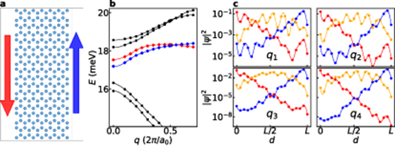
A zoom of the resulting energy dispersion, around the Dirac energy, is shown in Figure 4(b). The red and blue diamonds indicate modes that are exponentially localized at either edge of the ribbon, as shown in figure 4(c). For comparison, we also show (in orange) the wave function coefficients of a magnon mode that is not localized at either edge. Our results strongly indicate the existence of localized modes at the CrI3 edges, across the entire one dimensional BZ. Around the Dirac point these edge modes are chiral, and their energy is inside the gap. Their chirality is evidenced by the locking between spatial localization and propagation direction: all modes localized at a given edge have velocities with the same sign. Away from the Dirac point their dispersions are not linear due to the presence of long range exchange.
Figure 4. Magnons in CrI3 nanoribbon. (a) Sketch of the Cr sites of the ribbon unit cell. The iodine sites are not shown, for clarity. The red and blue arrows indicate the direction of propagation of the edge modes. (b) Dispersion of the ribbon magnons, zoomed at the energy of the Dirac gap. The data highlighted in red and blue belong to the edge modes. (c) Probability density for the edge modes (red and blue) as a function of the distance d from the left edge of the ribbon, for various wave vectors: q1 = 0.40,  , in units of 2π/a0, where a0 is the length of the ribbon's unit cell (
 times the monolayer lattice parameter). We also show in orange, for comparison, the probability density for a non-edge mode. The data plotted in red and blue match those for the corresponding branches in (b).
Download figure:
Standard image High-resolution image
4. Summary and conclusions
By using an itinerant fermion theory, we have shown that magnons in CrI3 can be computed without the use of spin models. We have presented strong evidence that magnons in monolayer CrI3 are topological, namely the existence of gaps, controlled by spin-orbit coupling, at the Dirac points, the finite Berry curvature with the same sign at all Dirac points and the braiding behaviour of the magnon eigenvectors along a line connecting different Dirac points. We supplement the evidence gathered in the monolayer by showing that a CrI3 nanoribbon supports chiral states along its edges, in accord with the principle of bulk-edge correspondence.
We would like to offer some perspective on the possible experimental detection of CrI3 magnons' topological features. First, as a result of the finite Berry curvature, magnons contribute to the thermal Hall conductivity at zero magnetic field [24]. Second, a specific consequence of the quantized Chern number is the existence of edge modes. Our calculations show they have narrow spectral features. Therefore, their existence could be confirmed by inelastic electron tunnel spectroscopy carried out with a scanning probe [47] to determine the local density of states of spin excitations with atomic resolution.
Our method to obtain the magnons directly from a microscopic electronic Hamiltonian derived from ab initio calculations is widely applicable to 2D materials and their heterostructures. The method can also be used to obtain spin excitations from non-collinear and non-coplanar ground states and to examine the stability of competing states, which can prove extremely useful in unveiling the nature of the magnetic ground state of Kitaev materials such as α-RuCl3.
Acknowledgments
We acknowledge useful discussions with M Costa, R B Muniz, A Molina-Sánchez and D Soriano. N M R P acknowledges support from the European Commission through the project 'Graphene- Driven Revolutions in ICT and Beyond' (reference No. 881603 – Core 3), and the Portuguese Foundation for Science and Technology (FCT) in the framework of the Strategic Financing UID/FIS/04650/2013, COMPETE2020, PORTUGAL2020, FEDER and the Portuguese Foundation for Science and Technology (FCT) through projects PTDC/FIS-NAN/3668/2013 and POCI-01-0145-FEDER-028114. J F-R acknowledges financial support from FCT UTAPEXPL/NTec/0046/2017 project, as well as Generalitat Valenciana funding Prometeo2017/139 and MINECO Spain (Grant No. MAT2016-78625-C2). D L R S thankfully acknowledges the use of HPC resources provided by the National Laboratory for Scientific Computing (LNCC/MCTI, Brazil). A T C thankfully acknowledges the use of computer resources at MareNostrum and the technical support provided by Barcelona Supercomputing Center (RES-FI-2019-2-0034).
Footnotes
- 5
A file with the hopping matrices used to produce the results shown in figure 1 is available as supplementary material.
- 6
Because of the very large computational cost, we have not tried a complete integration of the BZ.