


ABSTRACT
We develop a nonlinear dynamo model that couples the evolution of a large-scale magnetic field with the turbulent dynamics of a magnetofluid system in the small scale by electromotive force. Because the dynamo effect takes place in astrophysical objects characterized by a range of dynamical parameters (Reynolds numbers, Prandtl number, etc.) which is beyond the current possibilities of direct numerical simulations, we describe the nonlinear behavior of the system at small scales by using a shell model. Under specific conditions of the turbulent state, the field fluctuations at small scales are able to trigger the dynamo instability. The stability curve derived from our simulations allows us to gain some insight not only into the regime of parameters analyzed up to this point but also for very large Prandtl numbers. Moreover, from our analysis, it is shown that the large-scale dynamo transition displays a hysteretic behavior revealing its subcritical nature. The system, undergoing dynamo transition, can reach different dynamo regimes depending on the Reynolds numbers of the magnetic flow. This points out the critical role that turbulence plays in the dynamo phenomenon. Moreover, in this Letter, we show the presence of the natural ordering of dynamo regimes (oscillatory–reversing–steady dynamos) observed in the large-scale magnetic field for increasing magnetic Reynolds numbers. However, the signature of these regimes is also found in the small-scale dynamo by looking at the scaling properties of magnetic fluctuation energy as a function of magnetic Reynolds number.
Export citation and abstract BibTeX RIS
1. INTRODUCTION
One of the most fascinating and challenging topics in physics and astrophysics is the understanding of the generation and self-sustaining property of magnetic fields in planets, stars, galaxies, etc. The most accredited mechanism is the so-called dynamo effect, i.e., the maintenance of a magnetic field against diffusive effects by the motion of electrically conducting fluids. This effect has been studied in laboratory liquid metal experiments like Riga and the Von Karman Sodium experiment (Gailitis et al. 2000, 2001; Monchaux et al. 2007; Ravelet et al. 2008). Moreover, a full understanding of the turbulent dynamo problem is extremely relevant for explaining magnetic field generation in a fusion plasma device such as reversed field pinch (see Lorenzini et al. 2009).
The dynamo effect occurs because magnetic field lines are generally stretched at small scales by the random motion of the fluid in which they are almost "frozen." The stretching of the magnetic lines leads to an exponential amplification of the field until the back-reaction (via the Lorentz force) causes the saturation of this growth. A small-scale dynamo is generated when the system reaches energy equipartition at small scales. During the growth of the magnetic energy at small scales, the velocity and magnetic field fluctuations interact with each other, generating an electromotive force (e.m.f.) able to produce a large-scale magnetic field. The latter increases due to the turbulent fluctuations at small scales until a saturation level is reached.
Although direct numerical simulations (DNS) of MHD equations play an important role in our understanding of the dynamo problem (Kagemayama et al. 2008; Li et al. 2002), the parameter regime characterizing the natural dynamos is still beyond the power of today's supercomputers. The main attempt to overcome the limitations in the Reynolds number range covered by DNS consists of deriving from MHD equations a set of statistical equations using closure hypothesis as the eddy-damped quasi-normal Markovian approximation (Pouquet et al. 1976). Along the same lines, Kazantsev (1968) developed the so-called Kazantsvev–Kraichnan dynamo model, which is essentially based on a quasi-normal closure hypothesis of the induction equation, assuming given statistics for the velocity field. This model has recently been generalized and analyzed by several authors (Kulsrud & Anderson 1992; Subramanian 1999; Schekochihin et al. 2002), also reaching Reynolds numbers up to 107–108 (Malyshkin & Boldyrev 2009, 2010).
From the point of view of studying dynamo action for very large Reynolds numbers as well, shell models, originally developed to describe nonlinear MHD turbulent cascade (Frick & Sokoloff 1998; Giuliani & Carbone 1998), have also been used (Benzi 2005; Sorriso et al. 2007; Ryan & Sarson 2007; Benzi & Pinton 2010; Nigro & Carbone 2010). More recently, we developed a new shell model to describe the coupling between a large-scale magnetic field and small-scale turbulence described by using a shell model (see also Nigro et al 2011; Perrone et al. 2011). This model reproduces the dynamo effect driven solely by turbulent fluctuations, in the absence of a mean flow (α2-dynamo). In fact, even in the absence of the macroscopic shear, the α effect can give rise to dynamo action. This effect seems to play a decisive role for planetary magnetic fields as a geomagnetic field, in the fully convective stars, and it may provide a possible mechanism for explaining magnetic activity, along with a nonaxisymmetric field as observed in many active stars (Meinel & Brandenburg 1990).
In this Letter, we present this new dynamo model focusing our study on the dynamical transition toward the regimes where the large-scale magnetic field is generated. Dynamo transition results from an instability: when the magnetic Reynolds number Rm reaches a critical value Rmc, the magnetic field releases its stability from a quasi-zero-magnetic field state generating the initial exponential increase until the dynamo quenches. Generally, the dynamo bifurcation could display at least two different natures: subcritical and supercritical (Manneville 1990; Morin & Dormy 2009), in analogy with turbulent transitions. We also investigate its nature, using our model developed with the aim of overcomeing the limitations in the Reynolds numbers range covered by current DNS.
2. NONLINEAR DYNAMO MODEL
Steenbeck et al. (1966) suggested that the net effect of averaging many small-scale turbulent motions would be to produce a large-scale electric field (α effect) generating a large-scale magnetic field. In the same spirit, we generate a decomposition of the fields in an average part, varying only on the large scale L, and a turbulent fluctuating part, varying at small scales ∼ℓ, with the assumption ℓ ≪ L (Biskamp 1993). Performing this scale separation, we obtain, in the induction equation in the large scale, a term which describes the action of small scales on the large ones consisting of a turbulent e.m.f. This can be written in terms of the Fourier modes of velocity (u(k, t)) and magnetic field (b(k, t)) small-scale fluctuations as follows:

which is a correlation between velocity and magnetic field fluctuations at small scales.
Introducing a basis in the complex spectral space:  ; and writing expression (1) in a form symmetric with respect to the change of k in −k (hence, the sum is over half k space), we finally find
where u1 and u2 (b1 and b2) are the components of u(k, t) (b(k, t)), along  and
and  .
.
At large scales, we consider an axisymmetric situation where a large-scale magnetic field can be decomposed into a toroidal and a poloidal component with respect to the symmetry axis. Moreover, we limit this to a local analysis where we can approximate the toroidal ( ) and poloidal (
 ) unit vectors with the Cartesian unit vectors, respectively,
  and
and  . Hence, the field at large scales is

where Bϕ and Bp are the toroidal and poloidal components of the magnetic field, respectively.
We describe the nonlinear dynamics at small scales by a Sabra shell model, in which the wave vector space, where one considers the small-scale dynamics, is divided into a finite number N of shells of radius kn = 2nk0 (with n = 0, 1, ..., N; and k0 ∼ 2π/ℓ is the fundamental wave vector). In each shell, complex scalar variables un(t) and bn(t) are assigned, describing the dynamics of velocity and magnetic Fourier modes in the shell of wave vectors between kn and kn + 1. The nonlinear coupling of neighbor shells is chosen in such a way as to conserve total energy, cross helicity, and magnetic helicity and to avoid unphysical correlations of phases. We can write the set of self-consistent equations for our dynamo model in which the e.m.f. is in a form consistent with the shell model:
where Bp and Bϕ fulfill the same equation ( ). These equations are in dimensionless units: the field fluctuations are measured in terms of a typical Alfvén velocity cA, the time is normalized to 1/(k0cA), the lengths are normalized to 1/k0, and finally, ν and μ, the dimensionless viscosity and magnetic diffusivities, are normalized to cA/k0. The spatial derivative associated with large scales is estimated by dividing by the typical large scale L, n is the shell number, and fn is an external forcing term applied on the first shell (n = 0) of the velocity equations. This forcing has the role of ensuring an energy injection on the velocity field fluctuations (this is the same used in Nigro & Carbone 2010 with correlation time equal to 1 unit time). The first terms on the right-hand side of Equations (5) and (6) describe the effect of the large-scale magnetic field on the small-scale turbulent dynamics. Let us note that, exactly as in the corresponding MHD expression (1), the turbulent e.m.f. tends to vanish when the system evolves toward a state of strong correlation between velocity and magnetic field, characterizing the Alfvénic fluctuations (Dobrowolny et al. 1980).
The model equations (4)–(6) are numerically solved using a fourth-order Runge–Kutta scheme, considering L = 10 and varying ν and μ in different simulations. At the beginning of each simulation, we let the system become turbulent at small scales, i.e., we keep B = 0 up to 1000 unit times. During this time the energy grows at small scales. After that, when we are sure that the turbulence is fully developed, we introduce a magnetic field seed of amplitude 10−10 at large scales and we check whether the dynamo effect starts to develop.
3. NUMERICAL RESULTS
The numerical results reveal a strong sensitivity of the model with respect to the magnetic Reynolds number Rm ≃ δu/μ and a dependence on the hydrodynamic Reynolds number Re ≃ δu/ν, with δu being the rms of the dimensionless turbulent velocity. Depending on these parameters, the system evolves toward different scenarios: (1) no dynamo, (2) oscillatory dynamo, (3) magnetic reversals, and (4) steady dynamo. The transition from an oscillatory dynamo to a steady dynamo, going through a reversal regime, are obtained by increasing Re and Rm (Figure 1). The apparently counterintuitive fact that a higher Rm leads to a more regular dynamo (via the transition oscillatory–reversing–stationary; see also Figure 2) seems to be a generic feature of α-dynamo, like that studied by Stefani & Gerbeth (2005). The ordering of regimes, obtained here, is due to μ, which also influences the rms of  . Once the dynamo effect is developed,
  reaches a statistically stationary state in which the small-scale field fluctuations play the role of destabilizing
  from its average value, causing magnetic reversals or oscillations. The larger the rms of
  is (smaller μ), the more difficult it will be to destabilize
  , therefore, the probability of changing sign for
  will be smaller. On the contrary, this probability increases for a smaller rms of
  (large μ) causing reversals. For even larger values of μ one gets oscillations of
  .
.
Figure 1. Time evolution of the large-scale magnetic field in dimensionless units in different simulations. The system starting from oscillatory behavior undergoes the transition to reversal regime and finally reaches a steady dynamo for increasing values of the Reynolds numbers.
Download figure:
Standard image High-resolution image
Figure 2. δb/δu for increasing Rm in semi-log scale. Starting from no magnetic field state, we check the values of δb/δu during the running time of the simulation in which we increase Rm for ν = 10−5. During this time the system undergoes dynamo transition (magenta circles) reaching the oscillatory regime; afterward the system moves toward the reversal regime (black triangles) coming to a steady state (gray squares).
Download figure:
Standard image High-resolution imageIn order to better characterize the different regimes, we have performed a simulation with a fixed value of ν and changing the value of μ after a time interval sufficiently long with respect to the dynamical evolution times and we have studied how the parameter δb/δu changes for increasing Rm. The function δu/δb illustrated in Figure 2 shows a zero-order discontinuity corresponding to dynamo transition (the step for Rmc = 67) and a first-order discontinuity corresponding to the transition from oscillatory dynamo to reversal regime. The order of these discontinuities marks the different nature of the corresponding transitions; in particular, we can argue that the dynamo effect occurs as an instability while the other transitions occur with continuity. For Rm > Rmc, the parameter can be represented through a scaling law

where A and γ are the fit parameters. The fact that, in correspondence to the transitions from oscillatory to reversal and from reversal to steady state regimes, which are observed in the large-scale magnetic field, the scaling exponent γ changes its value showing that the different behavior of the large-scale field also has a direct influence on the small-scale turbulence and is extremely relevant. Moreover, it is worth noting that the steady state regime for the large-scale magnetic field is finally obtained when the turbulent magnetic field fluctuation amplitude has reached its maximum value, corresponding to equipartition between kinetic and magnetic field fluctuating energies.
Our model allows us to study the dynamo instability inside a very large range of values of critical parameters such as those found in astrophysical phenomena, but not yet accessible by DNS. For instance, in the interstellar or the intracluster medium Pm ≫ 1, in the Sun's convective zone, Pm ∼ 10−7 to ∼10−4, in planets Pm ∼ 10−5, and in protostellar disks Pm ≪ 1. Therefore we have investigated the dynamo threshold for different values of the magnetic Prandtl number, reproducing the stability curve in a very wide range of values, as illustrated in Figure 3. It shows a weak increase of Rmc for increasing Pm−1 > 1. This behavior is in agreement with Schekochihin et al. (2005), while other authors (e.g., Iskakov et al. 2007) claimed to approach a constant limit for the asymptotic behavior of Rmc for decreasing Pm. Probably the issue concerning this asymptotic behavior is not conclusively closed because a realistic parameter regime is still beyond the current possibilities of DNS and lab experiments. Concerning the other limit for large Pm, Figure 3 shows a strong monotonic increase of Rmc for decreasing Pm−1 < 1. The reason for this strong increase could be related to the need to have small magnetic diffusivity to compensate for the large viscosity in order to have small-scale field fluctuations large enough to consistently trigger the e.m.f. at large scales for the dynamo onset. On the one hand, this result is consistent with that obtained by other models in a smaller range of critical parameters: Pm−1 ∈ [1, 100] (Schekochihin et al. 2005; Brandenburg 2001; Ponty et al. 2005; Brandenburg 2009), giving us the possibility to be confident in our model, and on the other hand, it extends these results to a larger range of values not previously investigated.
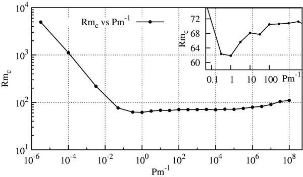
Figure 3. Stability curve Rmc vs. Pm−1(=Re/Rm) in log scale. The inset in semi-log scale shows a slight increase in Rmc for increasing Pm−1 > 1.
Download figure:
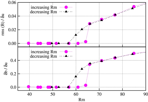
Standard image High-resolution imageThe dynamo onset could take place in a subcritical or a supercritical way. In some models and experiments it is subcritical, as shown in some small-scale dynamos, revealing a hysteretic behavior (Sahoo et al. 2010; Ponty et al. 2007). In order to investigate the nature of this instability as described in our model, we have reproduced hysteresis cycles realized as follows: for a fixed value of ν, starting from a state of a quasi-zero-magnetic field characterized by low Rm, we have dynamically increased Rm during the simulation time in order to destabilize the system from the initial state. During the simulation we have checked the time evolution of the order parameters: the ratio between the rms of  over δu and δb/δu. Only after a critical value of Rm, corresponding to the threshold for the dynamo action to get set up, have we found an increase in the large-scale magnetic field (first phase). Once the dynamo sets in, we have decreased Rm (second phase). In the second phase, order parameters do not follow the inverse path to the first phase, realizing a hysteresis loop. We have investigated hysteresis cycles considering a wide range of values of ν down to 10−11. For the example reported in Figure 4 where ν = 10−5, starting from a quasi-null magnetic field, we have increased Rm up to Rmc = 67, corresponding to the dynamo threshold, by finding the values shown by the magenta circles for the order parameters. After the dynamo onset, Rm keeps increasing, and the system displays magnetic oscillations and subsequently magnetic reversals. Once these regimes are reached, we have decreased Rm. The values of the order parameters, represented now by the black triangles, lie on the same curve of the first phase when the system is in the latter regimes; afterward the order parameters lie on a different curve starting from Rmc to lower values. This shows the hysteretic behavior of the transition and its subcritical nature. We have also found a slight suppression of hydrodynamic turbulence during the transition (Cattaneo et al. 1996), revealed by the decrease of Re. In the example in Figure 4, Re, starting from a value ∼8000, slightly decreases to 7000 when the dynamo action sets in. We can argue that the subcritical nature of dynamo bifurcation could originate from the reduction of turbulence due to the growth of the magnetic field, which ensures maintainence of the dynamo effect for lower Rm values.
Figure 4. Hysteresis cycles of  (top panel) and δb/δu (bottom panel) obtained around the stability margin of the bifurcation for the simulation with ν = 10−5 and changing Rm: we increase Rm reaching dynamo onset in which the magnetic field displays oscillations (1st phase: magenta circles), afterward we decrease Rm (2nd phase: black triangles).
Download figure:
Standard image High-resolution image
4. CONCLUSIONS
In conclusion, we developed a self-consistent nonlinear dynamo model, which solves the induction equation in local analysis at large scales, while the turbulent dynamics at small scales is described by a shell model. We point out that there is no prescribed form (like the α-term) for e.m.f., but it is consistently described by the form obtained using a shell model. Moreover, at variance with other dynamo shell models (Nigro & Carbone 2010; Benzi & Pinton 2010), which use ad hoc terms to mimic the dynamo instability, this model is able to reproduce different regimes in a dynamical way. In fact, an important result of this research is related to the critical role that the turbulence plays in the dynamo phenomenon showing how different regimes are obtained depending on Reynolds numbers of small-scale turbulent flow. In particular, we have shown the not obvious and apparently counterintuitive fact that a higher Rm finally leads to a more regular dynamo (via the transition oscillatory–reversing–stationary dynamo). One of the strengths of our model, due to the use of the shell technique, consists of the capability to describe the dynamo transition in a very large range of values of the Reynolds numbers, reproducing some results of the dynamo transition which are consistent with other models in the parameter range accessible to them, therefore showing its reliability. Moreover, in a parameter range (Pm−1 ≪ 1) which is not yet accessible to DNS and, to our knowledge, has not yet been explored by models based on a closure hypothesis, it predicts a peculiar behavior for the stability curve which would require confirmation by other approaches. Moreover, the study on the dynamo transition shows its subcritical nature supported by hysteresis cycles around the stability margin of the bifurcation. Finally, on the basis of the results presented here, we believe that this model can provide a contribution to the understanding of the dynamo problem due to its capability to cover a larger range of values not yet accessible by DNS, but more realistic for natural dynamo processes.