
Abstract
In recent years, machine learning and deep neural networks applications have experienced a remarkable surge in the field of physics, with optics being no exception. This tutorial aims to offer a fundamental introduction to the utilization of deep learning in optics, catering specifically to newcomers. Within this tutorial, we cover essential concepts, survey the field, and provide guidelines for the creation and deployment of artificial neural network architectures tailored to optical problems.
Export citation and abstract BibTeX RIS

Original content from this work may be used under the terms of the Creative Commons Attribution 4.0 license. Any further distribution of this work must maintain attribution to the author(s) and the title of the work, journal citation and DOI.
1. Introduction
Deep learning (DL) is a subset of machine learning (ML) that uses deep neural networks (DNNs) to solve complex optimization problems [1–3]. Unlike traditional analytical approaches, DL is particularly useful when there is little knowledge about the underlying system or when there are many degrees of freedom that make predicting outcomes difficult. In such 'black box' scenarios, DL can be trained using inputs and outputs alone, without the need for explicit knowledge of the system's inner workings.
Before the advent of DL, another optimization approach with similarities to DL was evolutionary algorithms (EAs) (the best known of these are genetic algorithms) [4, 5]. EA and DL are both optimization approaches that can handle complex problems without requiring a complete understanding of the underlying system. EAs are inspired by natural selection and use techniques like mutation and crossover to evolve solutions over time. In contrast, DL uses artificial neural networks to learn from large datasets through repeated forward and backward propagation.
This tutorial focuses on the use of DL for solving various problems in optics with an emphasis on providing guidelines on how to choose the right DNN architecture for specific problems and on how to implement it. The decision-making process for solving optics-related problems using DL is illustrated schematically in the concluding figure of this tutorial: figure 11. As shown in the diagram, researchers must address two primary questions when building a DL model: 'Do I have data?' and 'What architecture should I use?'. Subsequently, the flow chart outlines the sequential steps involved in constructing an appropriate model for a given optical problem. Throughout this tutorial, we will describe the different strategies mentioned in this diagram.
In the context of this tutorial, we mention that an important emerging subject by itself is the development of optics-based neuromorphic engines. In other words, using optical systems for performing neural networks' operations. Such solutions can be based, for example, on diffraction or on integrated nano-photonics [6–10].
The structure of this tutorial is as follows: in section 2, we start by introducing basic concepts in DL to establish a common language for the remainder of the tutorial. Then, in section 3, we provide guidelines for choosing and applying DNN architectures for different problems, and demonstrate these with specific examples. Afterward, in section 4, we provide a detailed overview of the many different problems in optics for which DL has proven useful while commenting on the applied architectures used for some of these problems. In passing, we also mention some optic-based implementations for DL algorithms, i.e. designing an optical system that implements some target DL task, such as classification for example, achieving, therefore, optical computing. Finally, in section 5, we make some general conclusions and provide our thoughts on the future of this field.
2. DL: the basics
In this section we will discuss DL foundations, focusing on DNNs. The goal of this section is to give the reader information on the basic components used in common architectures of DNNs (such as layers and non-linear functions), the data setup, how DNNs are trained and optimized, and some helpful know-hows and rules-of-thumb that will assist a beginner to get started with exploring the optimal architecture for their task. More details may be found in [11, 12]. Readers familiar with the field may proceed directly to section 3.
2.1. Basic layers
DL algorithms are based on DNN architectures. A DNN consists of a large number of layers of various types, such as convolutional layers, fully-connected (FC) layers, recurrent layers, transformers, etc (to be described shortly). Each layer contains numerous nodes called neurons, which are learned (optimized) weights. Neuronal architecture is inspired by biological models of neurons in the brain. In figure 1, we can see a schematic comparison between a biological neuron and the neuron used in neural networks. Every neuron in the brain has multiple inputs called dendrites and the neuron outputs a signal to other cells as a function of the inputs via the axon terminals. In DL, the artificial neurons receive multiple inputs and calculate their weighted sum (while the weights are learned as we will explain later, in section 2.5), and then output a single value following a non-linear function.

Figure 1. Biological neuron vs. computational neurons. On the left, a representation of a biological neuron with its dendrites at the top. The dendrites input signals into the neuron and following some thresholding operation a signal will be propagated through the axon to the axon terminals where it will be sent to other neurons. Similarly, on the right, a computational neuron gets multiple inputs from other neurons. It calculates their weighted sum and following some non-linear operation,  , it outputs a signal to other neurons.
Download figure:
Standard image High-resolution imageEach layer has its own unique collection of traits and characteristics.
2.1.1. FC.
The FC layers, shown in figure 2, connect every neuron output from the previous layer to all the neurons of the next layer. This configuration grants every neuron access to all the previous neurons' data while allowing it to weigh their importance for its own output result. Note that an FC layer uses maximum connectivity (from all previous neurons to all the neurons in the next layer), which may be inefficient for a large number of neurons and for large dimensions of data. This transform can be described as dense matrix multiplication and bias vector addition. Namely,  , while the matrix
  and the bias vector
  are learned weights, and
  is the input vector (or a vector from the previous layer). The pre-defined parameters (hyper-parameters) of this layer are the input and output dimension sizes and should be defined while creating the network before the optimization. Hyper-parameters, in general, are a set of parameters used to control the learning process of the network [1].

Figure 2. Fully-connected layer. A schematic representation of a fully-connected layer. Each layer has a certain set of neurons, in this case indicated by circles, and each one of those neurons is connected to all other neurons from the previous layer's neurons. The lines between the neurons signify the connections between the different neurons and their widths signify the weight given to each connection. These weights are learned iteratively. Each neuron takes the weighted sum of the previous neurons and passes it through a non-linear function.
Download figure:
Standard image High-resolution image2.1.2. Convolutional layers.
Unlike the FC layers, in the convolutional layers, shown in figure 3, the spatial relation between neighboring values is utilized. This type of layer will use a set of kernels or filters in 1/2/3 dimensions (usually sized  ,
,  , or
, or  for two-dimensional (2D) image kernels) that will be convolved with the output of the previous layer, aiming to extract different features from it. This allows the layer to be indifferent to the input size while having fewer parameters than the FC layer. Since the kernel is small it extracts only local features from the input signal. Therefore it is usually used for time-series (one-dimensional (1D)), images (2D) and videos or three-dimensional (3D) volumes (3D). For example in two-dimensions, this layer is computed as
  , while the kernel
  and the scalar b are learned weights, and
  is the input image (or features from the previous layer). Any layer's input data consists of single or multiple channels of different features. Each layer usually consists of multiple filters applied to the input, which calculate different types of features. The set of all features is known as the 'feature map'. Each element in the feature map represents the response of the corresponding filter to a specific region of the input. Formally, the output feature map
 ![$j\in[1,C_{o}]$](https://content.cld.iop.org/journals/2040-8986/25/12/123501/revision2/joptad08dcieqn12.gif) is computed as
is computed as  for
for  , number of input and output channels respectively. The convolution kernel tensor in such a case is
  . Usually we use
 ![$k_1 = k_2 \in [3,5,7]$](https://content.cld.iop.org/journals/2040-8986/25/12/123501/revision2/joptad08dcieqn16.gif) .
.

Figure 3. Convolutional layer. A schematic representation of a convolutional layer. Each layer has a certain set of learned weights that are saved inside a kernel. The kernel will be passed over the input, multiply each pixel by the weights, and then pass the sum of the weights through a non-linear function. The kernel output is considered as the feature map of the kernel. Convolutional layers usually include numerous kernels. The kernels' weights are learned iteratively during training.
Download figure:
Standard image High-resolution image2.1.3. Recurrent layers.
In contrast to the previously discussed layers, the recurrent layers constitute an entirely distinct category of elements. Unlike the other layers, a recurrent layer consists of a singular unit that unfolds over time, with its weights being progressively trained across various temporal intervals. The iterative training of weights occurs as the unit unfolds over time (see figure 4). Through the utilization of recurrent layers, temporal information can be encoded, thereby enabling the concealed temporal distribution of the data to be learned by the network. The significance of recurrent layers extends across numerous domains involving time-dependent data, exemplified prominently within the realm of natural language processing (NLP), time series analysis, robotics, and many more [13].

Figure 4. Recurrent layer and attention layer. A schematic representation of a recurrent layer and its unfolded representation over time. The trainable layer 'A' is shared across timesteps and controlled by internal 'state' information passed between timesteps. The attention layer consists of mathematical operations on the extracted  features from the data (using fully-connected layers) to bring attention to the most valuable correlations in the input data.
Download figure:
Standard image High-resolution image2.1.4. Attention layers.
The attention layer selectively focuses on important input elements based on the attention mechanism. This layer was introduced for NLP [14] with state-of-the-art results and adopted also for computer vision tasks [15]. In this layer, the computed correlations in the input are dependent on the input data itself, unlike previous layers where the kernels were independent of the input (e.g. convolution kernel). The correlations are computed by a dot product of 'key' and 'query' vectors which are learned from the input data. After normalization, these matching scores are considered as weights for the 'value' learned vectors. It can be expressed using the equation  , where
  is the queries matrix that contains query vectors representations of n elements,
  is the key matrix that contains key vectors representations,
  is the value matrix, and
  are the dimensions of the representations. The keys, queries, and values are computed from the data using FC layers. For a schematic representation, see figure 4.
2.1.5. Common blocks.
The DNN is usually built from several blocks of layers, including weighted layers (FC or convolution) normalization (e.g. batch-normalization) and activation functions. The residual block is a common convolution block and was first introduced in the ResNet architecture [16]. This architecture consists of two pairs of a convolution layer followed by an activation function. The input data is added to the second convolution result before the last activation function. This skip/residual connection of the input to the output increases significantly the deep network's performance by allowing the gradients to back-propagate more easily without the vanishing gradient problem (will be discussed in section 2.5). The dense block [17] consists of several convolutional layers where each layer obtains inputs from all its preceding layers, and passes on its computed feature maps to all subsequent layers. In contrast to the residual block, in this architecture the features are not summed before they are processed by a layer. Instead, they are concatenated along the feature dimension.
2.1.6. Other layers.
The division of the network into layers allows each layer to learn a different representation of the input data—the deeper the layer is, the more abstract its representation could be [18]. The output of the last layer is also the output of the entire network. It could be a scalar value, a vector, a matrix, or even a tensor of a higher dimension (could be considered a matrix with extra dimensions), depending on the data and functionality we want our network to learn. A neural network could also include more types of components, such as dropout [19], max-pooling, average-pooling, batch-normalization [20], skip-connections [16], etc. Each one of these components has its own functionalities and can be used at different locations along the network. It is essential that you understand what each component of your network does before building it in order to correctly train and use it. For example, a pooling operation reduces the spatial dimensions of a feature map by selecting representative values (via taking the maximum value in an area, max pooling, or taking the average, average pooling), aiding in extracting key features while decreasing computational complexity.
2.2. Non-linear activation functions
The layers are usually separated by non-linear activation functions, which extend the network's capability to optimize for not only linear functions, while the target real-world function (it tries to learn) is assumed to be non-linear. If non-linear activation functions were not present, the entire network would consist of a concatenation of linear operations. Therefore, it is simply a linear function and can approximate only linear functions which are just a subset of all existing functions. By adding non-linear activation functions, however, the linearity of the network is broken and we can approximate a solution to more complex non-linear problems. There are a couple of desired qualities for activation functions. We would want our activation functions to be zero-centered so that they would not shift the output of each layer in any specific direction, thus, preventing bias. In addition, we want our activation functions to be differentiable. This is because, as we will see later (in section 2.5), the whole learning process is based on an algorithm known as back-propagation which is dependent on the fact that the whole architecture of the network is differentiable. There are many activation functions. The most commonly used ones, shown in figure 5, are the sigmoid function— , the hyperbolic tangent (tanh) -
  , and the rectified linear unit (ReLU) - ReLU
 [21, 22]. Each activation function has its own pros and cons and is used in different scenarios. The sigmoid function is not commonly used inside the network due to the fact that it is not zero-centered and saturates very quickly toward 1 or 0, therefore diminishing the network gradients very quickly. However, in case we know that our output is limited between 0 and 1 (as is the case, for example, with probabilities), it can be used at the network output. The hyperbolic tangent, on the other hand, is zero-centered and usually performs better than the sigmoid inside the network.

Figure 5. Activation functions. Three examples of activation functions are presented. From top to bottom: sigmoid, tanh, and ReLU functions. The ReLU function has no upper limit, while the sigmoid and tanh functions are both limited in the range of [0,1] and [−1,1], respectively.
Download figure:
Standard image High-resolution imageThe chosen activation function can affect the performance of the neural network and so when one designs a neural network one should research the possibility of different non-linear activation functions. Most often, for classification problems, the output layer of the entire network will be activated by a function from the Sigmoid family, since we are seeking probabilities of classes. The most commonly used one for this type of problem is the Softmax function— , since the output is a probability vector, namely, with non-negative values that add up to one.
The ReLU function is not zero-centered but is very easy and quick to calculate and does not suffer from the vanishing gradient problem (a known problem in ML, which will be discussed in 2.5, and can prevent the training of a neural network). The fact that it is time-efficient and works well makes ReLU the most commonly used activation function nowadays [1]. In most cases, your first try for an activation function should be ReLU.
2.3. Normalization layers
Normalization layers are used to improve the optimization process and the network performance by normalizing the features during the forward pass of the data into the network. The transformations applied to the data consist of first normalizing the data, and then rescaling it using learned mean and standard deviation. Using such transformations in the network after processing layers (FC, convolution, etc) contributes to consistent statistics of the computed features for different data samples at the specific location of the network (which usually have different features statistics). Such an approach helps the network converge and achieve improved results. The most commonly used normalization approach is batch-normalization [20], which normalizes each feature in the network independently across the input samples. Formally, in batch-normalization, each feature is normalized as  where µx
and σx
are the mean and standard deviation of x respectively. Then, the data is scaled by
where µx
and σx
are the mean and standard deviation of x respectively. Then, the data is scaled by  using learned parameters γ and β which are optimized during training. Other common normalization approaches include group-normalization [23] and layer normalization [24]. When the batch size (in stochastic gradient descent (SGD) as described below) in the training of the neural network is large, batch-normalization should be preferred. Yet, if a small batch is used (typically smaller than 16), group-normalization usually leads to better results.
2.4. Optimizer and loss functions
When we design the specific architecture we believe will work well for our problem, we also have to carefully design two more important functions—the optimizer and the loss function. We want to optimize the network weights for the desired task by reducing the loss of the network. The loss function evaluates the error of the network (like a cost function) according to the task performed. Using the loss function, gradients are calculated with respect to the network weights. These gradients are used to update the network weights using a first-order optimization method (commonly called the optimizer).
2.4.1. Optimizers.
The basic optimizer of neural networks is SGD. Gradient descent is a fundamental optimization algorithm used to minimize (or maximize) a function by iteratively adjusting its parameters based on the gradient's direction. The goal of gradient descent is to find the minimum (or maximum) of a given function by moving in the direction of the steepest descent (or ascent) along the gradient of the function. When many training samples are given, gradient descent first evaluates the error of all of them and only then calculates the gradients and performs one descent (or ascent) step. SGD is a variant of this algorithm that at each iteration evaluates the error of only one randomly selected sample and performs the gradient update based on it. This improves convergence efficiency during the training process, especially when dealing with large datasets. Yet, the gradient directions in SGD are ʼnoisy' as they are calculated based on only one sample each time. To alleviate that, SGD is commonly used in mini-batches, i.e. the gradients are calculated on multiple randomly selected samples instead of a single one. When using an optimizer there are some parameters that should be set. The learning rate, which is the step size of the gradient steps, is such common parameter.
The purpose of the optimizer is to update the weights and thus, reduce the loss and increase the accuracy of the network. To improve the optimization process, one may add regularization to the used loss function, e.g. in the form of weight decay (an additional constraint on the network weights), or improve the optimizer. One such approach is using momentum, which considers the previous steps of the gradient descent for a more stable convergence. The most common optimizer today is Adam [25], which is generally regarded as being fairly robust to the choice of hyper-parameters [1].
2.4.2. Loss functions.
The loss function is a function used for measuring the distance between the ground-truth output for the network (the actual, correct, or true values of the target variables that the network is trying to predict or classify) and the output predicted by the network after feed-forwarding the input sample related to this specific ground-truth output, throughout the network. The learning process aims to minimize the loss function. Some of the loss functions are designed for solving classification problems, where the output can be defined as a label from a finite set of labels. Others are designed for solving regression problems where the objective is to establish a relationship between input features and a target variable, where the target variable is a continuous quantity that can take any value within a certain range. Commonly used loss functions are—mean squared error (MSE), mean absolute error (MAE), categorical cross-entropy (usually used for multi-class classification problems) and binary cross-entropy (suitable for binary classification problems)—many other loss functions are expansions or derivatives of the ones mentioned here [26]. Different problems require different loss functions. Usually, we use MSE and MAE when solving regression problems, in which we try to minimize the error and get as close as possible to the real (ground-truth) value. For example, in image transformation problems, we would prefer to apply MAE, as although it is 'slower' on its way to a minimal loss, once the distance gets smaller than one, its steps are still significant, unlike MSE, which will get 'stuck' there. Classification problems are more probability oriented, thus it is recommended to use loss functions from the cross-entropy family, which aim to reduce entropy between different, related, or non-related values, such as probabilities that sum up to 1.
2.5. Back-propagation and training
We covered the general architecture of a neural network, but one of the most important parts of a DL algorithm is the way it learns. DNNs learn by optimizing the network parameters using an algorithm called back-propagation [1], which essentially computes the gradients needed for employing gradient descent in an artificial neural network. In general, the learning process proceeds as follows—the network feeds forward a number of input samples, called a mini-batch, and predicts the outputs (conditioned by the network weights). It then compares the output and the ground-truth using the loss function. Then, in the back-propagation step, the gradients of the weights and biases of the network are computed backward (from the output back to the input, using the chain rule) and each parameter in the network is optimized according to the optimizer algorithm (a variant of gradient descent), aiming to converge to the global minimum of the loss function after a sufficient number of forward–backward (optimization) iterations. Due to the non-convexity of the function, the network usually converges to a good enough local minimum. Feeding the network with all the data once is called an epoch. Since feeding large datasets is costly (in terms of memory, processing time etc), the data is split into mini-batches for the forward–backward passes. We usually train the network for a number of epochs and sometimes randomize the data samples between epochs, in order to create different mini-batches for each epoch which improves the stability of the learning process. Following the training of the network, we will maintain the network's weights constant and check its performance. If we see that our network does not converge, or does not give good enough results, we will tweak the network's architecture (e.g. number of layers, number of neurons in each layer, types of layers, activation function), training method and hyper-parameters (e.g. data, loss function, learning rate, optimizer type, etc) and run the whole training process again in order to get a better result. While performing back-propagation, it is important to be mindful of vanishing gradients and exploding gradients. Vanishing gradients occur when a neural network's gradients become exceptionally small during training, causing sluggish convergence and impeding learning. Conversely, exploding gradients manifest as exponential gradient growth, resulting in numerical instability and posing difficulties updating model parameters effectively. Various techniques have been developed to address these issues [16, 20, 27], including skip connections, which will be further explored in section 2.8.
2.6. Data setup
When working with a new data set we usually split the data into three subsets: training set, validation set, and test set. The training set, as the name suggests, will be used for training the network in small batches. Some of the data (usually 10%–30%) is taken out before training and serves as the validation set at the end of every epoch. The purpose of the validation set is to determine whether the network has converged and learned relevant features for data it has not trained on, so their loss function values should be similar. The test set is used to test the network's performance at the end of training. The test set will be a part of the data that the network has never seen during training and it will serve as the ultimate test for our network. Our goal is to train the network to effectively generalize from the training set to any data distribution, resulting in optimal performance for new data samples that it has not yet encountered. Thus, the data should be large and versatile enough to represent all possible cases. The data should be balanced and represent all cases equally. For example in classification, all classes should have the same amount of samples. When the data is imbalanced, bias will be added to the model. As an extreme example, consider a classification task where all the dataset is from a single class 'A'. In such a case, the model will learn to predict this class 'A' regardless of the input sample since, during training, the model was optimized to output only 'A'. Moreover, inaccuracies in the data may harm the performance of the model. In particular, inaccuracies such as false labels/samples or domain differences. False labels or samples will add 'noise' to the training process and may decrease the model's performance. Thus it should be eliminated as much as possible from the data during the labeling process or during the creation of data samples. Domain difference is caused when the training data is different from the testing or real-world data, and the drop in performance is called a 'domain gap'. This situation is common when the model is trained on simulation data or data from a distribution different from that of the target (such as occurring from measurements from a different setup/sensor). Assuming the model learned to generalize well in the training domain, it may gain poor performance on real-world samples. To eliminate (or reduce) this phenomenon, we should aim for data distribution which is as close as possible to the real-world distribution.
Normalization of the input data may improve network convergence since all samples have the same characteristics. Normalization relates to the numerical values representing the data. Thus, one can normalize the data using the mean and standard deviation of the samples, or normalize the dynamic range of the samples. Normalization can be helpful not only for the input data but for the input of every layer. One very common method is batch-normalization, which we also mentioned above. Batch-normalization is a technique in DL aimed at improving the training stability and convergence speed of neural networks. It involves normalizing the intermediate activations within a mini-batch of training examples, reducing internal covariate shifts, and allowing for more efficient gradient propagation. This normalization process helps mitigate issues like vanishing and exploding gradients, leading to faster and more stable neural network training.
2.7. Overfitting and underfitting
During training, we will want to watch out for unwanted effects such as overfitting and underfitting. Overfitting will usually occur if our model has more parameters than needed to learn the data, and so it will be able to find a model that will fit exactly with the training set while not generalizing to the validation set. Appropriately, with underfitting the issue is exactly the opposite, the model is too small and so cannot fit and cover the complicated data distribution. A good indication of overfitting will be that the loss value for the training set becomes much lower than the loss value for the validation set (or the loss value for the validation set starts to diverge). On the other hand, for underfitting, the loss for the training set gets stuck at a value that is insufficient for the problem we are trying to solve. In figure 6 these two effects are depicted, where an underfitting situation can be observed at the top of the figure, indicating that the data distribution, presented in the inset, was not adequately captured by the model. Consequently, the training and validation losses did not converge to a low level. In the second row, a representation of overfitting can be clearly seen, wherein the model converges into an excessively complex model that fails to generalize to the validation set, as indicated by the noticeable gap between the training and validation losses. Thirdly, on the bottom row, a 'good' training outcome is depicted, wherein the model has converged to an acceptable loss level (lying between the underfitting and overfitting cases) while maintaining its generalizability and discarding some outliers in the process.

Figure 6. Underfitting and overfitting. Three examples of three possible training outcomes. In each row we can see in the inset the different data points clustered in a two-dimensional space, where each color indicates a different class. The trained model separation criteria are indicated with the green dashed line. From top to bottom we can clearly see the three different cases for underfitting (train loss is high), overfitting (train loss is low but validation loss is high), and regular fitting (both train and validation losses are small), respectively. The loss plots show the validation and train losses throughout the training process and exhibit different convergence behaviors.
Download figure:
Standard image High-resolution imageIn order to avoid both effects, we can try to adjust the complexity of our model or use the validation set to check when to save the weights for our model. There are numerous published techniques that try to deal with overfitting and underfitting, such as early stopping, dropout layers, pruning, and many others [28]. We would use early stopping when we believe there is a certain threshold of loss or accuracy we have to achieve. After achieving said threshold, we would like to save the model and weights and stop the training process. Dropout is another method for preventing overfitting, where at each step, the dropout layers randomly select (using a threshold probability) which neurons will be used, and which will be deactivated without changing the network architecture. This way the network makes each neuron 'learn' more features, making it more robust to changes. When using dropout layers you should make sure that the dropout is performed only during training and not in the validation or test phases. Another method for preventing overfitting is pruning, where we optimize the model, removing neurons we believe are redundant. For the case of overfitting, one obvious possibility is to increase the amount of data. One way to increase the amount of data without actually labeling and measuring more data, which is an expensive and time-consuming process, is to use a process called data augmentation. In data augmentation, we can use our data set and extract more data from it by using features that we think are independent of the labels. For example, if we are working on classifying cats, we should be able to classify the cat regardless of its orientation and so we can add a lot of samples to each sampled image by simply rotating it.
2.8. Network architectures
There are many types of DNN architectures. Here we will address the most commonly used ones. The simplest neural network architecture is an FC network. This type of network consists only of FC (also known as dense) layers, connected by activation functions (usually ReLUs) and normalization layers (usually batch-normalization). The second type commonly used for images and sequential signals is a convolutional neural network (CNN). This type of network consists of many convolutional layers connected by activation functions and normalization layers. The network size is defined by the amount of layers (depth of the network), and by the width of each layer, namely the amount of features. In classification tasks, at the deeper end of the network, usually there is an FC part, which takes the flattened vector output (a 1D vector representing or converted from a multi-dimensional array or matrix) of the last convolutional layer and extracts a vector or scalar output. The rise of CNNs has changed the computer vision field entirely, giving state-of-the-art results for image classification challenges, such as the ImageNet challenge [29]. Commonly used CNNs are VGG-16 [30], MobileNetV2 [31], ResNet [16], and more. Another type of CNN is the fully-CNN (FCNN), which consists only of convolutional layers, allowing the network to be indifferent to the input size of the network, in contrast to networks that contain dense layers, which constrain the input size. FCNNs are usually used for image-to-image translation problems.
Encoder–decoder architecture is an architecture of two networks. One is an encoder that encodes the input data into a lower dimension using several layers or blocks. The second is a decoder that remaps the low-dimensional encoded data back to the input dimensions [32], and these networks are trained together. An architecture of this type creates a bottleneck in the flow of data along the network, making it possible to extract useful information from the data through the network. The architecture can be trained in an unsupervised way, such that the reconstructed data by the decoder will be the same as the encoder input. In such a case, the data is compressed into a low dimensional space, which can be used for different requirements. A very commonly used FCNN is U-Net [33], which is an encoder–decoder convolutional network, used in many fields. The encoder part of the network reduces the data resolution (usually by a factor of 2) several times to a lower scale. The decoder upscales the resolution the same amount of times to the resolution of the original (input) data. One of the most important features in the U-Net architecture is the skip-connections that concatenate the features from the encoder to the decoder at each resolution level. These connections between layers in a neural network enable the network to retain and combine information from different depths. As a result of skip-connections, U-Net is able to capture intricate local details and broader context simultaneously, making it possible to jointly encode and decode data, while also avoiding gradient vanishing, allowing for more efficient training and better feature extraction. In recent years, 3D CNNs have also started to be in use, allowing the analysis of videos and 3D data and not only images, using 3D convolution kernels. A commonly used one is C3D network [34], but there are many more being developed, as analyzing time-series data, like videos, keeps being a very interesting and not yet solved problem.
Many different problems in DL use the same building blocks we discussed above for different types of problems. For example, object segmentation and detection can both be considered a classification problem of sorts with some important spatial information and so a CNN or an FCNN could be relevant. Noise filtering can also be considered an image-to-image transformation and so an FCNN will also be relevant here. Generative adversarial networks (GANs) uses an architecture to train generative models (see section 3.6) to generate new data examples. This architecture is trained in a special configuration where two networks compete against one another to optimize a loss that is a combination of their combined goal [35]. One part of the network, the generator, tries to generate fake samples that look real enough to the other part of the network, the discriminator. The discriminator tries to figure out whether the new data is fake or real. Despite this network architecture appearing more complex, the basic building blocks remain the same. For example, if you design a GAN that generates experimental data from a simulation, your generator architecture could be an encoder–decoder architecture based on an FCNN. The loss might be slightly different than with a regular FCNN that performs segmentation, for instance, but the building blocks will stay the same. The training of such an architecture might be unstable and the diversity of generated images might be limited. Therefore, some variations were suggested to improve stability and results [36, 37]. The evolution and architectural layout of these different networks are depicted in figure 7. The figure presents the architecture of an FC network that has undergone evolutionary changes, resulting in the emergence of a CNN on the right side. The CNN incorporates convolutional layers that effectively utilize spatial information. Furthermore, the utilization of an encoder–decoder architecture in an FCNN for addressing image-to-image tasks is depicted. As already explained, the encoder takes in the input data and maps it to a lower-dimensional or compressed representation while the decoder generates a desired output at a higher dimension from the encoded representation. Moving to the bottom panel, the figure portrays a common architecture of a GAN. In this architecture, a generator is constructed using the same building blocks as the FCNN, albeit without the inclusion of the encoder section. Additionally, a discriminator employing a CNN architecture is employed to discern between fake and real samples. This illustrates that various network architectures are constructed using shared building blocks.

Figure 7. Neural networks types. The depicted illustration showcases the evolutionary progression of distinct neural network architectures. Commencing with the earliest and fundamental fully-connected network, which exclusively employs fully-connected layers as previously outlined. Subsequently, the convolutional neural network (CNN) emerges, incorporating convolutional layers primarily while still incorporating fully-connected layers toward the end. Following that, the fully-convolutional neural network (FCNN) is presented, where the fully-connected component has been completely eliminated. Lastly, the generative adversarial network (GAN) architecture is illustrated, which amalgamates the aforementioned architectures and involves a distinctive training procedure employing two networks to facilitate the generation of synthetic data. In this figure, each square represents a data matrix whose size is proportional to the matrix size. The array of yellow small squares represents data after encoding into a lower dimensional space. In the FCNN a decoder follows the encoder and it enlarges the data into a larger dimension.
Download figure:
Standard image High-resolution imageMore intricate paradigms, such as reinforcement learning (RL), use different configurations of classifiers to train and implement a controlled process where an agent can perform under real-life conditions. The network architecture is trained to output an action for the agent trying to maximize a reward function and this action is performed by the agent while the network 'keeps track' of the agent's surroundings and state and adjusts accordingly [38]. For example, a helicopter will learn how to fly and do tricks on its own while getting inputs from its physical environment [39], or an agent will learn how to predict a protein structure [40], or AlphaGo which introduced a combination between Monte-Carlo tree search and 'value' (value functions help the agent evaluate the desirability of states or actions) and 'policy' neural networks (which define the agent's decision-making strategy) to beat even the most professional of Go players [41]. This type of network could be very helpful when you wish to formalize a strategy and a set of actions while interacting with the environment. This is different from, for example, a classifying CNN which does not adapt to new inputs from the environment.
Although still uncommon in optics, transformers are a relatively new type of DL model that is starting to be used in many fields of research, mainly in NLP and computer vision. Transformers were first introduced in the paper 'Attention Is All You Need' [14]. They are based on a sequence-to-sequence encoder–decoder architecture and were initially commonly used for language translation problems [42, 43]. The transformer model introduced innovation in the way it utilizes attention mechanisms to improve different tasks. This can be demonstrated by using translation problems: imagine reading a sentence—a contextual sequence of words—each word is more strongly related to some words in the sentence than others. The transformer's attention model will give more significance to such words.
Transformers are now commonly used in many types of tasks in computer vision [15, 44] and have helped make significant advancements in the field of video understanding, as videos are sequences of images (or frames). As we mentioned above, this tool is not yet common in optics. However, it has a lot of potential for many types of problems that might not have closed analytical solutions.
3. Guidelines for choosing and designing a neural network
When designing and training a neural network for a given task there are several aspects to consider. These depend on the background knowledge available on the target task and the amount of data available.
If lots of data are available and the input–output data is similar to a common task, then one may just pick a state-of-the-art architecture according to the task and data, such as EfficientNet [45] or ResNet [16] for image classification tasks or U-Net [33] usually for image-to-image tasks. Yet, in some cases, it might be difficult to train such models from scratch due to a lack of data and not having enough diverse samples. This may lead to poor results by the neural network. To this end, several approaches can be utilized, such as transfer learning and data augmentation, as described in the following subsections. The network and training can have different schemes, such as supervised or self-supervised training, algorithm unfolding, generative models, etc. These are described below.
3.1. Transfer learning
Transfer learning is a method of transferring a pre-trained model for some close task or domain (namely source) to the desired task or domain (namely target). It is commonly used where there is not enough data to train the model from scratch, and it enables achieving better results than training a model from scratch. It can also be used to speed up the training process. The source domain is preferred to be as similar as possible to the target domain, and the tasks should also be similar to get better performance. To make it possible, both the trained model weights and the architecture structure should be available (e.g. online on GitHub.com). Probably several training approaches should be considered and evaluated using the validation and test sets to find the most suitable method for the task.
3.1.1. Entire model training.
Assuming the source model architecture is suited for the target task, for example, image-to-image translation (using an FCNN network) or classification with the same number of classes, we can use the pre-trained source model and resume training on the target domain. Since the target dataset is small, there is not enough data to train the model from scratch, but using pre-trained weights trained on a large dataset (the source domain) we can utilize the information embedded in the weights to achieve better results. Practically, we load the model with the trained weights on the source domain and resume training of the entire model (all layers) on the target dataset for several epochs, usually less than the full training process. The learning rate in this method might be low, such that the pre-trained model will be fine-tuned and will not tend to overfit the target domain.
3.1.2. Partial model training.
In some cases, we can freeze some layers in the pre-trained model, such that they will not change during training, and fine-tune only the rest of the layers according to the target domain. Given the idea that deeper layers in the network learn deeper features and are more task-related, while shallower layers learn simpler and basic features in the signal if the source and the target tasks are similar, we can freeze the initial layers and fine-tune only the last layers. For similar source-target tasks, fine-tuning only the last layer of the network (while the rest of the network is frozen) is a common practice. There are situations where we need to change the network architecture from the source task to suit the target task (for example in a classification where the number of classes in the source task is different than for the target). In such cases, we replace the relevant layer with a new layer with new characteristics (e.g. different output size). Due to the fact that this layer has not been trained previously, its weights may have been randomly initialized, and we will train it to fit the target task (for the classification example above, we change the last layer to fit the new number of classes and train it according to the target dataset and classes). The number of epochs and learning rate considerations are the same as in the previous subsection.
3.2. Data augmentation
Data augmentation is a method to increase the amount of data samples artificially. In this method, we use existing data samples and prior information about the data to generate new and different data samples. Usually, we perform an operation on a true sample from the dataset which guarantees that the sample characteristics are maintained (such as the label, semantic information etc). Some of the common methods for data augmentation are: shifting, rotating, mirroring, and scaling the signal. For example with tasks dealing with natural images (typically real-world images taken with a camera which are often complex and varied), we can shift the image and rotate it in small amounts, flip it horizontally, or zoom in, while the resulting image will still look like a natural image and maintain its content (label, for example, in classification). In contrast, notice that vertical flipping for natural images does not guarantee that the original sample characteristics will be preserved since the augmented image will not look like a natural image. Thus, augmentation operations should be chosen based on prior knowledge, sample characteristics, and the desired characteristics to preserve. During the training process, it is common practice to generate (augment) new samples on the fly, namely after reading sample data and before feeding it to the model, the augmentation transformations would be applied (usually using random parameters for the shift, rotation, etc). Using data augmentations, while in each epoch all the dataset is fed to the network, the model gets slightly different samples each time such that it prevents overfitting and improves the generalization. In this context, adding noise to the samples (e.g. additive white Gaussian noise (AWGN)) on-the-fly is an additional method to improve the model generalization (specifically noise robustness).
3.3. Self-supervised learning
Supervised learning, which has been discussed so far, uses labeled data to train a neural network to predict the correct output. This process typically involves the use of an optimizer algorithm to minimize a loss function that measures the difference between the predicted output and the true label. Unlike supervised learning, where the data samples are annotated or labeled, unsupervised learning has no explicit labeling or annotation. Instead, we use other prior information to supervise the learning process.
In self-supervised representation learning the goal is to train a network to generate good representations from unlabeled data such that the network will be later used for some target tasks such as object detection or classification (usually with a small number of annotations) [46–56]. For self-supervised learning, we use the data samples themselves to supervise the model, such as reconstructing the samples or parts of them. In this way, the model learns features and characteristics of the data, which are later used for the required task. For example, in GANs, unlabeled images are used as the ground-truth of the training to learn the distribution function of the data and generate new images (samples). In an encoder–decoder architecture, the data is used both at the input and the output of the network to get an encoded representation of the data.
3.4. Algorithm unfolding
Algorithm unfolding [57–72], which is also known as algorithm unrolling, has been shown to lead to computationally efficient architectures that can attain good performance also with a small number of labels. Among other optical problems, it has been shown to be useful in phase retrieval [73]. In the unfolding approach, an existing iterative algorithm for the target problem is being unfolded into a network of depth K that is equivalent to performing K steps of the iterative algorithm. Then, some of the parameters of the algorithm are being trained using standard network optimization where labels are used as the output. If the labels are unavailable, one may train the network to mimic the iterative algorithm's output when used with many more iterations and in this case the network mainly achieves an acceleration in solving this problem.
Note that applying the neural network in the unfolding strategy has the same complexity as applying the iterative algorithm for K steps. Yet, the trained network is expected to get better results with relatively fewer steps than the iterative algorithm, which typically requires many more iterations. Examples of parameters that can be learned in the unfolding strategy are the parameters of linear operations or some parameters of the non-linear functions used in the iterative algorithm. Notice that to optimize the unfolding algorithm, we need to be able to calculate the derivatives of each step in the algorithm. These derivatives are then used in the back-propagation algorithm for training the network. In many cases, after we unfold the algorithm and get a certain network structure, we can deviate from the original structure of the iterative algorithm and modify it for our needs, e.g. by replacing the used non-linear functions with other ones or adding batch-normalization.
3.5. Solving inverse problems using a trained denoiser
An interesting strategy for solving general inverse problems is the plug-and-play approach and its variants [74–91]. The core of this methodology is using a denoiser for solving the inverse problem iteratively. It is assumed that a denoiser exists for the type of data that is being handled. A denoiser is an algorithm (e.g. learning based such as a neural network) that removes noise from data, usually AWGN. Designing such an algorithm either by training or using a model is usually an easy task for most problems. Particularly, it is usually an easier problem than solving a general inverse problem.
The denoisers in this approach are used as priors and applied iteratively to solve the problem at hand. Usually, these strategies apply alternately a denoising step and a step for optimizing the inverse problem without the prior. The alternating minimization algorithm depends on the optimization strategy employed. Such strategies include half-quadratic splitting, projected gradient descent (where the denoising algorithm is considered as the projection), alternating direction method of multipliers, etc.
3.6. Generative models
GANs [92–94] and the recently proposed diffusion models [95–99] and normalizing flows [100] are strong models for learning in an unsupervised way data distributions and sampling them. These models transform a certain vector space, denoted as the latent space, which can be learned as done in StyleGAN [101–103] or GLIDE [104], into the space of desired generated images. The latent space has desirable properties, which allow performing manipulations on it, that can lead to solving inverse problems [105–111], to having a good representation for classification [112–117], or to intuitive image editing [118–124]. Specifically, for the classification task, the latent space of these models has been used for performing regression of some properties such as age or face pose from a small number of examples [113], for getting a consistent semantic segmentation of parts in generated objects for improving performance on real data [114–116], or for efficiently getting data annotation that leads to more efficient training [117].
Diffusion models [95, 98, 99, 104, 125] is a recent new method for image generation by iterative diffusion steps starting from Gaussian noise to a natural image. This method is more powerful and capable of generating better and more diverse samples than previous generative methods, but it requires more computational power. One of its common uses is data generation conditioned on input text, e.g. as in DALL-E2, Midjourney, or Stable-Diffusion. We believe that this capability can be used also in the physics realm in the sense that diffusion can be used to generate new physical models conditioned on some provided physical requirements or constraints.
3.7. Useful DL packages
The most popular way to use DL in practice is using Python with the PyTorch package [126]. It implements all the common neural network components with strong graphics processing unit (GPU) acceleration, which is very important in order to train and run the neural networks in a reasonable time. On top of PyTorch, there are several libraries that are very common for some specific applications. For example, the 'Hugging Face' Transformers [127], Diffusers [128] and PEFT [129] libraries are very popular for the use of transformers, diffusion models and efficient neural network fine-tuning, respectively. OpenMMLab gathers in a unified easy-to-use manner state-of-the-art computer vision open source models for many tasks such as object detection [130], semantic segmentation [131], object tracking [132], etc. Open3D [133] and PyTorch3D [134] are very popular for 3D data representation and processing. Gymnasium [135] and dopamine [136] are popular frameworks for RL. Fairseq [137] is a popular library for sequential data such as speech and language. Its pre-trained models and code can be useful when working with other types of sequential data.
4. Survey of the use of DL in optics
DL has proven to be an asset in many fields of physics, ranging from astrophysics to particle physics [138–141]. This type of development was expected since many problems in both fields use large amounts of collected and analyzed data and so DL can be used to recognize patterns or trends in the data much better than other computational paradigms. In particular, in optics, an assortment of different works appeared considering the possible usage and applications of DL algorithms. We can divide these works into two major trends. The first group of problems deals with solving optics-related problems with DL. The aim here is to take a well-established optical problem and check in what ways DL can be used to optimize its solution. Alternatively, DL can also be used to find solutions to optical problems that have not been solved yet. Within this group, we can find many different examples of problems from many different optics fields. The second group of problems deals with the other side of the coin. Instead of using DL to solve optics-related problems, optics will be used to solve DL-related problems.
4.1. DL for optics
In order to gain an appreciation for the work accomplished in applying DL for optical problems, a table is provided to the reader (table 1) which outlines the most cited works (as of the date of submission of this tutorial), in several fields in optics. Additionally, a set of doughnut charts is presented below, in figure 8, which divides the works conducted within this group of problems by network architecture and subtopic. Prior to diving into specific fields of optics that can benefit from the novelties DL algorithms offer, it is crucial to understand what makes optics data different, and why should one even consider using DL algorithms to solve optical problems in the first place. As mentioned above, visual data and time-series data are the natural types of data for DL algorithms, mainly the ones that are based on convolutional filters, which are the lion's share. Optics data can be represented well as visual or time-series data, depending on the problem we are trying to solve, and the field we are encountering. For example, imaging problems can be represented as an input image, and an output image, where the output image can go through any optical set-up we choose. In most cases of imaging problems, which are also prevalent in computer vision (denoising, dehazing, etc), one will try to take the output of an optical set-up as the input for the DL algorithm, and the input of the optical set-up as the desired output of the DL algorithm, trying to solve an inverse problem. That is: one would try to predict the required input to the optical set-up that creates a desired optical output. The same paradigm works for inverse design of nanophotonic structures, and other fields. One of the main shortcomings of DL algorithms, which one needs to take into account while designing a data set and a suitable neural network architecture, is that it is not trivial to generalize over input size in most types of problems. Classification problems, for example, where one might desire to classify optical data into a constant set of characteristics, present a constraint where the usage of an FC layer at the deep end of the network dictates a constant input size. This issue limits the degrees of freedom of a given optical set-up. Moreover, even if the network is fully-convolutional, thus, indifferent to the input size, its degrees of freedom would still be somewhat limited, as the sizes and number of its spatial filters are constant, usually dictating, at least, a range of different input sizes.

Figure 8. Networks distributions. The distribution of classes of networks utilized within each subtopic in the first group of problems, concerning the application of deep neural networks for solving optical problems, is presented above. It is evident that the distribution undergoes changes across various fields. As optical problems predominantly involve visual data presented in a two-dimensional space, convolutional neural networks (CNNs) and fully-convolutional neural networks (FCNNs) emerge as the most frequently employed network architectures across all fields. Notably, although generative adversarial networks (GANs) have been employed, they are not the prevailing approach. Interestingly, an outlier is observed in nanophotonics, where the fully-connected (FC) architecture is predominantly utilized. This is likely due to the parametrization of certain nanophotonics problems, which has led to the widespread adoption of this method.
Download figure:
Standard image High-resolution imageTable 1. Methods used in a select set of works that demonstrate the type of problems that are typically solved within different fields in optics.
| Field | Name | Reference | Method presented |
|---|---|---|---|
| Nanophotonics | Training deep neural networks for the inverse design of nanophotonic structures | [142] | Tandem architecture combines forward modeling and inverse design, addressing data inconsistency issues in training deep neural networks for the inverse design of photonic devices. |
| Deep-learning-enabled on-demand design of chiral meta-materials | [143] | Bidirectional neural networks is presented for efficient design and optimization of three-dimensional chiral metamaterials, enhancing prediction accuracy and facilitating the retrieval of designs, thus expediting advancements in nanophotonic device development. | |
| Imaging | Lensless computational imaging through deep learning | [144] | Deep neural networks (DNNs) for end-to-end inverse problems in computational imaging, enabling the recovery of phase objects from propagated intensity diffraction patterns using a lensless imaging system. |
| Deep learning microscopy | [145] | Enhancement of the spatial resolution of optical microscopy, expanding the field of view and depth of field, without altering the microscope design, by generating high-resolution images from low-resolution, wide-field tissue samples, potentially impacting other imaging modalities. | |
| Designing optical elements and systems | End-to-end optimization of optics and image processing for achromatic extended depth of field and super-resolution imaging | [146] | A novel research proposes a joint optimization technique, integrating the optical system design with reconstruction algorithm parameters using a fully-differentiable simulation model, leading to enhanced image reproduction in achromatic extended depth of field and snapshot super-resolution imaging applications. |
| DeepSTORM3D: dense 3D localization microscopy and PSF design by deep learning | [147] | Addressing the challenge of precise localization of densely labeled single-molecules in 3D, this study introduces DeepSTORM3D, a neural network trained to accurately localize multiple emitters with densely overlapping Tetrapod PSFs. This approach enhances temporal resolution and facilitates the investigation of biological processes within whole cells using localization microscopy. | |
| Other emerging fields | Machine learning approach to OAM beam demultiplexing via convolutional neural networks | [148] | CNN-based demultiplexing technique for orbital angular momentum (OAM) beams in free-space optical communication, providing simplicity of operation, relaxed orthogonality constraints, and eliminating the need for expensive optical hardware. Experimental results demonstrate its superior performance compared to traditional demultiplexing methods under various simulated atmospheric turbulence conditions. |
| Deep learning reconstruction of ultrashort pulses | [149] | The proposed deep neural network technique, validated through numerical and experimental analyses, enables the reconstruction of ultrashort optical pulses. This technique allows for the diagnosis of weak pulses and reconstruction using measurement devices without prior knowledge of pulse–signal relations. Successful reconstruction is achieved by training deep networks with experimentally measured frequency-resolved optical gating traces. |
4.1.1. Nanophotonics.
In the field of nanostructures, meta-materials, and nanophotonics in general, DL has become a prominent tool and a lot of different reviews were written on the synergy of these two different research fields [150–153]. We would like to point out the review by Khatib et al [152] for any newcomers to this specific field. The problems in this field can be divided into forward and inverse types. In forward problems, the network is trained to function as a fast simulator due to the high computational time required for simulating the interactions included in a specific nanostructure. This type of simulator will be highly useful in cases where the goal is to characterize the functionality of hundreds of structures, or in cases where some other optimizer will be used to solve inverse design problems. The more challenging and interesting problem is the inverse design problem. In this scenario, the network learns the reverse mapping between some target functionality and relevant device parameters. These types of problems are highly challenging since the design space does not always completely map the target space. More specifically, the most prominent problem is that, in most cases, the mapping from some structure to some target functionality is not a one-to-one mapping, and so the training process will not converge easily. In addition, some target functionalities can be impossible physically, and in some cases, there is no way to know that in advance while characterizing and designing the simulation or structure. Finally, some functionalities can be out of the scope of the training set and so the network will not be able to generalize to another set easily. The last two points can cause the network to give some solutions that are completely unrelated to the optimal solution for a target functionality.
To the best of our knowledge, most works in this field deal with the inverse design problem and not the forward problem. In some cases, the forward problem was only solved so as to be incorporated into a tandem solution. Using this approach, the forward network is used as a limiter for the design space and solves the one-to-one mapping issue that we have discussed previously [142, 143, 154, 157–159]. Most works in this field vary in two parameters, the nanostructure in question or the network used. Some works present the same solution for the same structure but with a different architecture. Choosing a specific type of a nanostructure and its representation will affect the network architecture design in the following stages. For example, when dealing with unit cells of a specific nanostructure we can choose to parameterize each unit cell in a certain way or decide on a completely unparametrized unit cell. A parametrized case is defined by a discrete set of parameters such as width, thickness, and permittivity. In contrast, an unparametrized case is described by a continuous distribution of the permittivity in space for example via an image. This choice will greatly affect what type of network should be chosen. For the parameterized case, since we have some vector with a set of parameters as output, the FC network is the obvious choice [160–162]. For the unparametrized case, where we have an image of the unit cell, convolutional layers will be required [155, 163, 164]. Both choices can cause design challenges. Parameterized designs can greatly limit the versatility of your training set while unparametrized designs are limited by the spatial sampling frequency of the grid of choice, and there is no clear-cut guideline to define the right approach. In figure 9 we can see an example of such a dilemma, both 9(a) [154] and 9(b) [155] deal with the same inverse design problem but the first uses an FC network, whereas the latter uses a decoder that outputs the image of the unit-cell. In our view, the solution to this dilemma lies in the choice of the nanostructure. For example, structures that require very high accuracy in their dimensions might be better off with the FC architecture, while structures that require high versatility to get a significant change in the output will require convolutional layers. Thus, returning to our initial point, you will effectively choose the correct network for the problem by choosing the representation for the nanostructure. But the network architecture is not the only thing we will need to choose. The loss function is of great importance as well for the success of the training process and its chances of generalizing to unseen data. Usually, in this type of problems, we will choose loss functions from the regression family, i.e. MAE or MSE. That is the obvious case for the parameterized nanostructure. For the unparameterized nanostructure, one might have more suitable loss functions to choose from. One prevalent choice can be the structural similarity index metric (SSIM) [165]. As its name suggests, a loss function based on SSIM calculates the similarity between two images, while minimizing the effects of minor displacements, rotations, noise, etc. The SSIM loss function between two images denoted by x and y is defined as follows -


Figure 9. Nanophotonics. Four different networks were used to find the correct nanostructure geometry for some target spectral response. (a) A fully-connected network that uses three inputs of the horizontal and vertical spectrum and the material's properties to predict the geometry. The architecture is based exclusively on fully-connected layers and has been designed specifically for this problem [154]. Reproduced from [154]. CC BY 4.0. (b) The same concept as the previous paper but with some convolutional layers that were added after a reshaping of the middle layer [155]. Reprinted with permission from [155] © The optical Society. (c) The architecture and results for a GAN are shown [156]. Reproduced from [156]. CC BY 4.0. (d) The results for another GAN architecture are shown [157]. We can clearly see that the results for both (c) and (d) were not always in the same orientation as the ground-truth. Reprinted (adapted) with permission from [157]. Copyright (2018) American Chemical Society.
Download figure:
Standard image High-resolution imageWith µx
the pixel sample mean of image x, µy
the pixel sample mean of image y,  the variance of x,
  the variance of y, σxy
the cross-correlation of x and y,
the variance of y, σxy
the cross-correlation of x and y,  ,
,  , two variables to stabilize the division with a weak denominator, with L being the dynamic range of the pixel values (usually
  while
while  and
and  , by default).
The utility of using such a loss function comes in problems where the solution might be indifferent, to some extent, to rotations, displacements, and noise.
Another consideration is which approach is better—using supervised or unsupervised learning. There is a clear benefit for using supervised methods as they are easier to train. Still, some works tried to solve the inverse design problem using unsupervised methods, such as GANs [156, 157], and RL [166]. The benefit of using unsupervised models is that the one-to-one mapping issue becomes an asset instead of a problem. Similar to the way a GAN can generate multiple images of different cats given one label of a cat, in our case, a GAN will generate multiple images of different structures given one target functionality. In figures 9(c) and (d) we can see some examples of the results given by a GAN network. It is clearly visible that two solutions can give very similar responses in this case. On the other hand, working with unsupervised models can be tricky. In the GANs case, for example, the models can suffer from model collapse (which is a case where the GAN gets stuck on a specific subspace of the data and is unable to generalize).
The take-home message in this field is to familiarize yourself with the data before designing the network. Ask yourself a couple of questions: What type of structures will I be using (maybe they are 3D and so you might need a 3D network [167])? Is the design space versatile enough? If not, consider data augmentation. What parameters affect the response? Should they be weighted somehow (in the loss for example) to give more weight in the training to subtle parameters? Can I reduce the dimensionality of the problem and if so at what cost? Are there some nonphysical solutions that may be used as a case study for my model? How much data will I need so that the network can get a wide enough view of the problem at hand? Is there a one-to-one mapping between the design space and the target space? If not, consider looking into different one-to-many solutions that are available [168]. This set of questions should assist you in finding the appropriate architecture for your needs.
4.1.2. Imaging.
Naturally, a tool like a DNN, which is most commonly used for image processing and computer vision tasks, can be used for various imaging problems in optics, usually using some kind of a U-Net-based network, as most problems discussed are image-to-image problems—reconstruction, denoising, deblurring, dehazing, super-resolution, and more. In the field of imaging, some works deal with reconstructing the required phase applied with a spatial light modulator (SLM) at a specific plane, from the intensity pattern on a sensor. It can be in a lensless setup [144] where the main artifact that needs to be overcome is diffraction, making it a rather simple task, or in a setup that consists of diffusers that generate a speckle pattern [169–172]. Other works that reconstruct the source phase pattern from a speckle pattern generated by light passing through diffusers integrate auto-correlation methods into DNNs [173]. One more prevalent method is to use a conditional GAN (C-GAN) to denoise an image [174, 175]. C-GANs can also be used for robust phase unwrapping [176]. In some works, instead of a diffuser, the reconstruction was of a speckle pattern generated by light passing through a multi-mode fiber [177, 178]. In general, it can be reconstructed from any scattering media [179–181].
The reason why it seems so natural to apply DL algorithms from the fields of computer vision and image processing to optical imaging problems is the fact that, in many cases, these are the exact same problems. Usually, in the field of computer vision many tend to study natural images, or medical images, taken with a camera or sensors (x-ray, CT, MRI, etc), while the same applies to optical imaging.
Many imaging problems in optics, as one can see in the examples presented above, in figure 10, focus on reconstructing a source image. In many cases, we know what target light pattern we want to achieve, but we do not have an analytical model to reconstruct it. To achieve it, we usually create a dataset of source images and run it through our optical setup, to get the resulting light pattern on the target plane, surface, or volume. If we have an analytical model of the system, we can build a simulated dataset by generating source-target pairs using the known model [185]. Once done, we have enough data for the network to learn how to reconstruct the source. We can choose the type of patterns we want to pass through the optical system, e.g. natural images, random patterns, etc. When used with these types of datasets and training methods, the network is able to predict the source patterns fairly accurately in many cases. Moreover, it can save the researcher the time and effort of trying to get the exact pattern they desire, and even making it possible in cases when there is no analytical solution at hand. When training the model on simulation data, a domain gap may occur, namely, since the training domain is different than the real-world data for testing and using the model it may cause a drop in the model performance, thus we should have data as close as possible to the real world. When all options to bridge the domain gap have been exhausted, adding noise (e.g. AWGN) to the data may increase the robustness of the model to changes in the input data, and as such it may perform better on real-world data. Note that using real data measured from an optical system is not problem free. First of all, capturing the data may take more time and effort since hardware equipment is involved. A domain gap can also exist in some cases, where the system is changed (including parameters such as distances, temperatures, alignments etc), so the system behavior is different from the one we optimized for. In addition, keep in mind that the measurement devices can add noise to the samples, leading to noisy obtained data. It may be beneficial to increase model noise robustness for the data at the input. This is realized by simply adding noise to the samples. However, this noise may, in turn, change the ground-truth data at the output of the model, which we usually want to be exact.

Figure 10. Imaging. Four different implementations of four different imaging problems are presented. In the 'imaging' example, a lensless imaging problem was solved using an FCNN that was trained to retrieve the image before propagation. Reprinted with permission from [144] © The optical Society. In the 'Autofocusing' example, a similar concept is seen, utilizing an FCNN architecture to retrieve the focused image and phase of a hologram. Reprinted with permission from [182] © The optical Society. In the 'super-resolution' example, an FCNN was used to produce higher-resolution images from low-resolution and wide-field systems. Reprinted with permission from [183] © The optical Society. Finally, in the 'Depth of field extension' example, the use of an FCNN was used to design a phase aperture coding element to overcome DOF limitations. These works were selected as representative examples for each respective field, but it is apparent that an FCNN of sorts was employed in all cases to implement the solution to the problem at hand. Reprinted with permission from [184] © The optical Society.
Download figure:
Standard image High-resolution imageAs mentioned above, in most cases of imaging problems, one would use a U-Net-based architecture, as it is the most popular one for image translation tasks. However, we believe that in the near future, image translation problems will utilize transformers at an increasing rate following the recent advances and state-of-the-art results with transformers for visual tasks [15, 44].
Besides choosing the correct U-Net-based architecture, one would be required to design a loss function that would work well with images that are much more sparse than natural images, such as speckle patterns. Since minimizing the loss relating to the difference between two images is a regression problem, and being aware that the data set contains mainly sparse images, one would want to stay away from using the classic MAE and MSE loss functions, as they will converge to a poor local minimum quickly, because most of the target image is black (meaning, no light intensity). One commonly used loss function for sparse images is the averaged cross-entropy (ACE) [170], represented by the following formula -

where g is the ground-truth pixel value, p is the predicted pixel value, and the average is over all N pixels. Here i enumerates the different pixels.
Another commonly used loss function for sparse images is the negative Pearson correlation coefficient (NPCC) loss, given by -

where  and
and  are the mean values of x, the ground-truth, and y, the prediction, respectively. n is the number of pixels in each image.
Both loss functions handle sparsity better than MAE and MSE, as they both average the correlation between pixels in the same coordinates, and not just calculate the loss over the entire image. That is, they are more sensitive to specific locations at which there are differences.
4.1.2.1. Auto-focusing.
Another common problem in imaging and specifically digital holography is autofocusing. In this task, instead of reconstructing stacks of images and finding the focal distance of the sharpest imaging, DL is used to estimate the desired focal distance [186]. It can also be done end-to-end using a U-Net architecture that recovers the phase pattern and reconstructs an in-focus input from a hologram [182]. Unfortunately, in this kind of tasks, where a model either estimates the focal distance, or entirely reconstructs the in-focus image, there are usually inherent constraints. As the network trains with samples of given images at different focal distances, it usually overfits, and has a hard time generalizing to images or distances it was not trained on. For unseen inputs, it might diverge from the patterns it was trained on, and 'hallucinate' outputs.
We believe that visual transformers might take this field forward and overcome the inherent issues of overfitting.
As for loss functions one should look into, for the end-to-end case, it seems that the most prevalent function is the SSIM loss [182], but we suggest trying averaged cross-entropy, and NPCC, which might yield similar or better results.
4.1.2.2. Super-resolution.
Another field related to general problems in computer vision is super-resolution. In this field, most optics-related studies focus on using simple tools, like mobile-phone cameras or commercial microscopes, and getting high-end results using deep-learning super-resolution algorithms. These works are usually based on training image-to-image neural networks, such as U-Net [145, 183, 187], C-GAN [188], and combinations of encoders and classifiers [189]. The super-resolution research in optics leans heavily on methods and insights from image processing. One of the most important insights is that natural images usually tend to have many repetitions at different scales in the image itself, making it easier for the network to converge into spatial features that might make it easier to achieve super-resolution. That is why most works in this field of optics tend to study biological tissues under a microscope [145], and natural images in general.
With super-resolution, it is highly recommended to start with loss functions such as MAE, MSE, and their derivatives as they are useful in cases where post-processing does not change the relative positions of objects. Using simulative data, the downscaling operator (reducing the size or resolution) applied to the high-resolution image should be similar to the real-world effect, otherwise, the model will suffer from a domain gap (because it is trained on inaccurate low–high resolution pairs). Hence, for example, using bicubic interpolation downscaling may not match the optical system and a performance gap in such a case may exist and should be checked for. Moreover, using generative models, the result may match the data distribution but may not be accurate according to the scene, namely, the model will generate content (frequencies) to make the image look sharper but it will not be accurate (known as perception–distortion tradeoff).
4.1.2.3. Depth-of-field extension.
Limited depth-of-field (DOF) is a known limitation in photography. To achieve an all-in-focus image (or extending the DOF) different optical changes were applied to conventional imaging systems to enhance the reconstruction results obtained using DL algorithms [184, 190, 191]. DOF and auto-focusing are computationally similar problems and so follow the same DL methods and have similar constraints. Thus one would want to follow similar rules-of-thumb and know-hows for both.
4.1.3. Designing optical elements and systems.
Optical elements and systems can be designed using DL for various applications. The optical or physical parameters of the system elements can be defined as learned parameters and optimized along with the DNN weights (for image reconstruction e.g.) using end-to-end optimization and back-propagation. For such methods, the imaging model of the system should be known and simulated from the learned parameters. This approach is also known as 'Deep Optics' [192–196] and is used for several applications, including DOF extension [146, 184, 191], depth imaging [197–200], computational microscopy [147, 201–203] and more [204–207]. The data in such learning must be from a simulation since the optical system parameters are unknown and the result should be simulated using known calculations. During training, a physical simulation model with the learned parameters is applied on raw data (e.g. sharp images) and the result is inserted into the reconstruction DL model. After training, the physical simulation block is neglected and its parameters are used to manufacture the physical system. The captured data from the implemented real-world system is inserted into the reconstruction model. Note the possible domain gap when training on simulative data and testing on real-world dataset.
4.1.4. Other emerging fields.
In the field of optical communications, an assortment of different works have emerged presenting the use of different network architectures to solve different optical communications problems [208]. The cases which are more optical in nature are usually related to visual data and implement a CNN. For example, some works deal with demultiplexing of orbital-angular-momentum using a classifier network [148, 209–211]. Additionally, DL was also adapted for problems in ultrafast optics, most of which deal with the reconstruction of pulse patterns [149, 212–215]. Since the problems, in this field, usually deal with transforming some 2D information (a 2D spectrogram trace for example) to 1D information, i.e. the pulse amplitude and phase, the network architecture is usually a classifier or an encoder that includes convolution layers at the input and the signal is processed into a vector at the output. Recently, some works emerged where problems related to coherent control of optical beams were tackled using DL algorithms [216–218]. In most cases, the problem is the design of a set of pulses beams to get some desired pulse or beam. The network architecture design is determined by the definition of the problem, just as in the previous cases. For example, in cases where the problem is the design of a set of phases in an image the relevant network will be a CNN [216].
4.2. Optics for DL
One major trend in recent research is the design of optical systems that implement neural network functionalities. The obvious benefits of such optical computers would be parallelism (the optical field can be the sum of many different modes at the same time, where each mode can be used to encode a different input to the same problem), fast computing (signals propagate at the speed of light), and a slim power budget. As we have mentioned before, in DL problems, the network needs to be trained first using some data and then some predictions can be made using the trained network weights (this process is also called inference). The majority of the works that attempt to create optical neural networks focus on the inference part of the problem. Namely, the network weights are pre-trained using a computer and then implemented optically. Most works manufacture optical phase masks that will implement the network's pre-trained weights [6, 7, 219–223], therefore, achieving a speed of light inference while also realizing something similar to an optical CNN. These works differ mainly in the type of non-linearity (in some cases there is no non-linearity), the domain at which they work (e.g. Fourier versus spatial domain), and the integration of electrical and optical components. Alternatively, in an attempt to create an optical FC network, some works implement DNNs in nanophotonic circuits while accomplishing inference [8, 224] and partial optical training [9]. Finally, some efforts were invested in implementing RL for an all-optical recurrent neural network [10].
5. Discussion
In a world where DL algorithms have become a commodity, used in almost every field of science, and where non-experts can yield significant results with tools such as ChatGPT, Stable Diffusion, and others—we believe it is crucial for a researcher in the field of optics to become familiar with these algorithms, the tools that utilize them, and the basics of what is happening 'under the hood'. The main reason is that tools based on ML are improving rapidly, and more and more ways are being found to make it easier for researchers to employ these methods for real world scenarios. We are witnessing a huge revolution that is just in its infancy, and it is expected to be similar in impact, if not bigger than, the introduction of coding to perform experiments in optics and analyze them.
As described at length in this tutorial article, there are many ways to utilize ML tools, and specifically DL tools, to solve optical problems. We described the major DL strategies used in optics today. Yet, there are, obviously, many DL tools that are still 'on the shelf', waiting for suitable problems in optics.
This tutorial is meant to give a newcomer to the field of ML who has knowledge in optics, a taste of what can be done with ML tools. We propose to use this article as a handbook focusing on rules-of-thumb and know-hows, but urge the reader to explore further and find new interfaces between optics and ML. Despite the successful application of DL to Optics there are still many challenges and limitations considering such applications. Throughout this tutorial, we have discussed some of these. Here we give a summary along with some additional pertinent points. First let us review some challenges:
- Data: training neural networks requires large amounts of data. In many applications it is hard to gather accurate data to train the networks.
- Domain gap: to overcome lack of data, in many cases the neural networks are trained using simulated data. Yet, in most cases, there is a domain gap between the real and simulated data. Therefore, there is a need to adapt the model trained on simulation to the real data domain.
- Complexity: as a rule of thumb, in most cases, larger neural networks lead to better performance. Yet, this comes at the cost of higher computational complexity, which also requires more energy. This may pose a challenge in some applications.
- Transferability: models trained on one optics research problem might not easily generalize to another due to the unique nature of different optical systems and phenomena.
- Interdisciplinary expertise: successful application of DL in optics research often requires collaboration between experts in DL and experts in optics, as understanding both fields is necessary to design effective models.
Next, let us review some of the limitations of applying DL in optics:
- Black box nature: DL models often operate as 'black boxes,' meaning they can make accurate predictions without providing insights into the underlying physical processes. This is a limitation when one wants to actually gain insight and understanding the of underlying mechanisms of a given problem.
- Data bias: biases present in the training data can lead to biased models. In optics research, biases can arise from the way data is collected, leading to inaccurate or skewed results.
- Lack of physical constraints: DL models might not inherently incorporate physical laws and constraints, which are vital in any physical research, optics being no exception.
- Limited generalization: DL models can struggle to generalize well beyond the range of data they were trained on. This limitation can be particularly pronounced when dealing with rare events or extreme conditions in optics research.
- Uncertainty estimation: DL models often provide point predictions without quantifying uncertainty. In particular for applied optics tasks it is essential to understand prediction confidence, which can be challenging to estimate accurately.
Note that these are some of the most obvious challenges and limitations in the field and there are more to explore.
To conclude, the utilization of DL in optics represents a rapidly growing area of research with numerous promising applications. Within this field, DL has been applied to diverse optical problems. These problems range from designing and optimizing optical components and systems to resolving imaging problems that have been traditionally tackled by traditional optical techniques. The effectiveness and precision of DL approaches to addressing optical problems depend on the availability of a sufficient amount of data. Yet, as discussed in this tutorial, even in the case of small data, DL can be effectively utilized. This tutorial is concluded with a flow chart, shown in figure 11, guiding the prospective user on how to implement a DL network for a problem in optics.

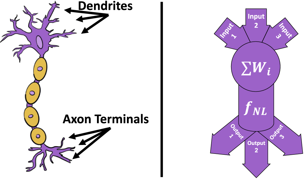
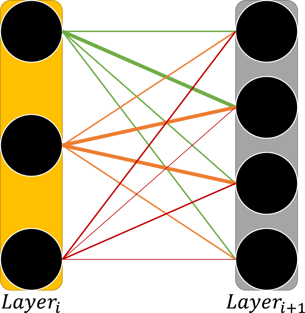
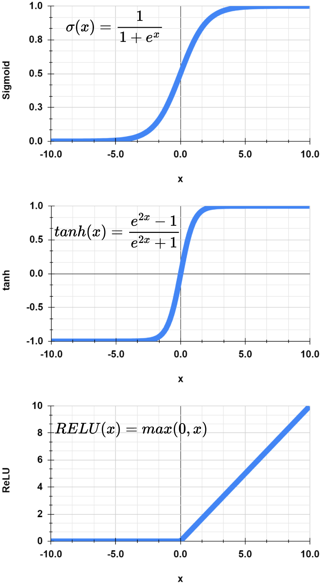
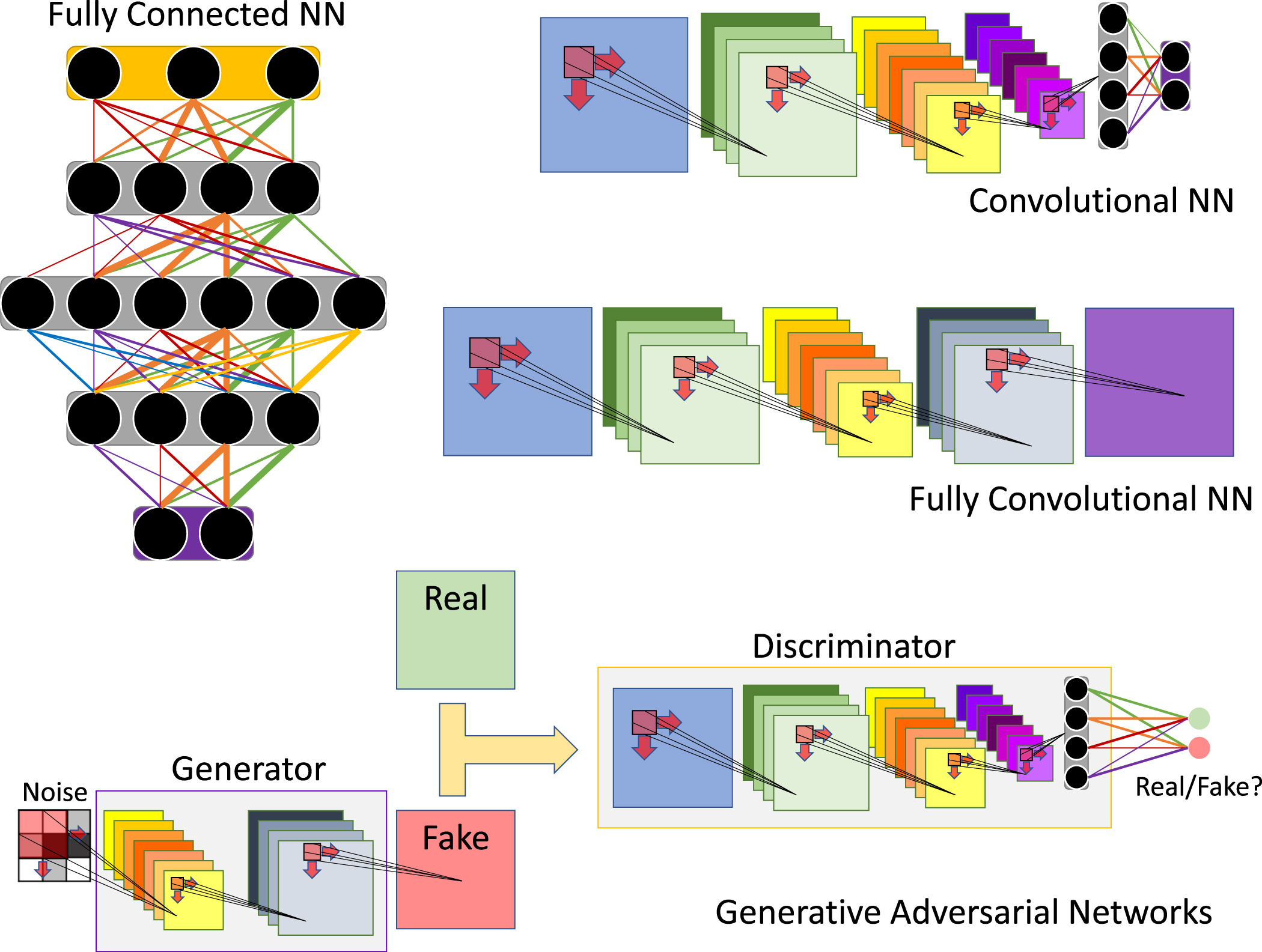
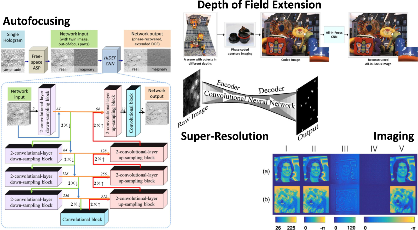
Figure 11. Flow chart for model training. The text within the cloud bubbles are different options that can be chosen for the boxed item to which they are attached.
Download figure:
Standard image High-resolution image
Data availability statement
No new data were created or analyzed in this study.
Funding sources
The authors received no specific funding for this work.
Conflict of interest
The authors declare no conflicts of interest.