
Abstract
The optical Archimedes screw is a structured beam of light shown to be useful in conveying airborne particles. Such beams were demonstrated propagating along straight and curved trajectories. Here we demonstrate an optical Archimedes screw where both its linear and angular momenta are accelerating—allowing to both control its trajectory and transverse profile during propagation.
Export citation and abstract BibTeX RIS

Original content from this work may be used under the terms of the Creative Commons Attribution 4.0 license. Any further distribution of this work must maintain attribution to the author(s) and the title of the work, journal citation and DOI.
1. Introduction
Optical beams that exhibit acceleration of an intensity lobe together with non-diffraction properties are a major area of interest for many years. Following the theoretical discovery of the Airy packet made by Berry and Balazs in 1979 [1] and the first observation of Airy optical beams in 2007 [2], an extensive interest in self-accelerating beams and their non diffraction property was initiated. A light beam is considered self-accelerating if it possesses an intensity lobe which traces a curve in space. Airy beams maintain a self-similar transverse profile along their propagation direction, a property which generally (and inaccurately) is referred to as 'non-diffracting' or 'diffraction-free' [3]. Bessel beams were first predicted and experimentally investigated by Durnin et al in 1987 [4]. Their non-diffraction property along with the axial symmetric transverse profile have drawn a lot of research interest to them. Bessel beams have another fascinating property of self healing, meaning the ability to reconstruct their shape after being disturbed by an obstacle [5]. Modifications of Bessel beams were shown to propagate in specific designed trajectories, e.g. spiraling and snaking [6–9], realizing acceleration.
A collaboration led by Efremidis, Christodoulides, and Chen has developed methods to realize self-acceleration of beams whose transverse profile can be described by a Bessel function of arbitrary order. These Bessel-like beams propagate in predesigned trajectories, both paraxial and non-paraxial [10–13]. Note that the directions of orbital angular momentum (OAM) and of the linear momentum change in space in such beams.
A few characteristics of Bessel beams of arbitrary order propagating in a straight line were shown to be controllable. It was demonstrated that the polarization state of the beam can be varied along the optical axis [14]. Furthermore, it was demonstrated that the intensity and hollow core radius of a Bessel beam can be tuned along the optical axis [15, 16]. Additionally, the intensity profile of Bessel beams with arbitrary trajectories can be tailored [17]. Other waves with interesting properties are Tornado and Galaxy waves that spiral with an accelerating rate of rotation [18, 19]. We refer the readers to two recent review papers detailing recent advances in this field [20, 21].
An interesting beam property is the modulation of the size of OAM with propagation. Beams with a varying OAM while propagating along a straight line have been suggested in a few publications [22–24]. Here, we treat the OAM as the value of the number l associated with the presence of the function  in the complex amplitude distribution of the beam, where
  . The direction of the OAM in this case is the direction of the axis around which a screw wavefront dislocation is formed. Note that for beams which are eigenstates of the OAM, l is the topological charge of the beam's singularity. Our beams, in most cases, are not such eigenstates, and so the formal association of the OAM with a topological charge in such cases is generally not valid [25–28]. In addition, the interpretation we use is a local one, associated with the distribution of the beam around an area of interest. In the same vein, we define the magnitude of the axial component of the local linear momentum as the value of the number k, associated with the presence of the function eikz
in the complex amplitude distribution of the beam, where z is the direction of the OAM as described above. In case the OAM is zero, the local momentum is simply the gradient of the phase of the beam.
. The direction of the OAM in this case is the direction of the axis around which a screw wavefront dislocation is formed. Note that for beams which are eigenstates of the OAM, l is the topological charge of the beam's singularity. Our beams, in most cases, are not such eigenstates, and so the formal association of the OAM with a topological charge in such cases is generally not valid [25–28]. In addition, the interpretation we use is a local one, associated with the distribution of the beam around an area of interest. In the same vein, we define the magnitude of the axial component of the local linear momentum as the value of the number k, associated with the presence of the function eikz
in the complex amplitude distribution of the beam, where z is the direction of the OAM as described above. In case the OAM is zero, the local momentum is simply the gradient of the phase of the beam.
Here, we demonstrate a beam with an OAM value that changes along propagation while the propagation trajectory itself is arbitrarily set. Thus both the linear momentum and OAM are accelerating in such beams. In particular the OAM is accelerating in both its magnitude and direction. A superposition of a beam with a varying OAM and a beam with a constant OAM, while both have the same trajectory, results in an intensity pattern curving in space with a changing amount of intensity strands. In fact, this is a further generalization of the optical Archimedes screw, a superposition of beams carrying OAM used to convey airborne particles along centimeter-scale straight or arbitrary trajectories in adjustable velocities and directions [29, 30]. The original optical Archimedes screw was a beam of light made of several entwined helical light-strands rotating around the optical axis of the beam [29]. The first generalization of the screw allowed the axis around which the strands were rotating to curve in space in an arbitrary manner [30]. Thus this screw was locally accelerating in space with regards to its local linear momentum. The current generalization, considered here, allows also for the local OAM carried by one of the beams comprising the screw to locally accelerate. There are several potential applications for the type of beams we demonstrate here, such as optical trapping and manipulation [31–34], OAM-based optical communications [35] and microscopy [36].
2. Results
2.1. Beam construction
Consider a superposition of two beams which differ in the magnitude of the axial component of their linear momentum and the magnitude of their OAM. Their interference results in both an axial and an angular standing wave patterns, combining to create a helical pattern. Using self-accelerating beams instead of beams propagating in a straight line keeps locally the principle of superposition of two modes with different linear and orbital angular momenta, while allowing their directions to change in space along a desired arbitrary trajectory. This was the idea behind the self-accelerating Archimedes Screw [30]. It was generated by a superposition of two Bessel beams with OAM values of 1 and 3 with different linear momentum along an arbitrary path. Both beams were designed separately according to an algorithm developed by Zhao et al [12] which created a curved vortex beam with a constant value of OAM. A generalization of the self-accelerating Archimedes screw allows engineering the OAM values along propagation in a curve to create a changing amount of strands in the interference pattern. Two Bessel-like beams are designed to propagate along an arbitrary trajectory, where one of them has a fixed OAM and the other one, an OAM that changes with propagation. To create such beams the input plane is divided into expanding circles, each one of them is mapped to a different axial value. The interference of rays emanating from these circles in the input plane leads to a Bessel-like pattern that propagates along the predesigned path. Further explanation for creating an appropriate phase pattern at the input plane as well as a code to implement it are given in [30] , which we adopted here. In order to vary the OAM with propagation each circle mapped to a different axial location is multiplied by the desired OAM function:  , where l can be any arbitrary number, integer or fractional. In this manner it is possible to tailor the OAM value at each axial location. We designed two optical Archimedes screws with varying OAM values, accelerating along a specified trajectory:
  (The units are given in meters.) The phase pattern at the input plane needed to realize the beams is shown in the left column of figure 1. The OAM as a function of propagation distance is set to be changing linearly for the first beam (first row) and step-wise for the second beam (second row). The middle column shows the OAM value as a function of propagation distance. A calculation using Fresnel field propagation shows iso-intensity surfaces of the beam in the right column.

Figure 1. Curved optical Archimedes screw with varying OAM. Top row: linearly varying OAM. Bottom row: step-wise OAM. Left column: the phase pattern at the input plane needed to realize each of the beams. Middle column: the predesigned OAM as a function of propagation distance for each beam. Note that each beam is comprised of two Bessel beams—one propagating along an arbitrary trajectory with a fixed OAM (in red) and the other propagating along the same trajectory while its OAM is changing (in blue). Right column: simulation of several iso-intensity surfaces of the beam relative to the beam's maximal intensity.
Download figure:
Standard image High-resolution image2.2. Experiment
The experimental setup consists of a 532 nm CW laser (Laser Quantum Ventus 532 Solo) which reflects off a phase-only spatial light modulator (SLM) (Holoeye Pluto SLM) following expansion and collimation. After the SLM the beam is demagnified with a collimating telescope and imaged using a scientific CMOS camera (Ophir Spiricon SP620U Beam Profiling Camera) on a translation stage set on the optical axis of the beam. The two phase profiles for creating the two beams (shown in figure 1) were multiplied with a blazed phase grating, directing a background free replica of the beam to the first diffraction order. The overall phase pattern, was loaded to the SLM which was set in a 4f configuration between itself and the imaging area. The measured intensities and extracted phases are presented for three axial locations for both the beam with the linearly varying OAM (figure 2) and for the beam with step-wise varying OAM (figure 3). The two top rows of each figure show the simulation results obtained using Fresnel field propagation, where the first row is the intensity and the second row is the extracted phase. The two bottom rows of each figure show the experimental results, where again the first row is the intensity and the second row is the extracted phase. The center of the white crosshair at the intensity plots indicates the position of the optical axis (at which passes the center of a beam propagating along a straight line). It can be seen that the experimental results are in good agreement with simulation results. In order to extract the phase from the experimental measurements we created three additional phase masks to realize the following fields:  ,
,  and
and  , where Ein
is the input field needed to generate the beams displayed in figure 1. For each of these fields, three intensity profiles were measured, added and subtracted to extract the phase, where
, where Ein
is the input field needed to generate the beams displayed in figure 1. For each of these fields, three intensity profiles were measured, added and subtracted to extract the phase, where  is the field Ein
after propagation to each of the imaging planes. The phase extraction procedure for each of the propagation distances is as follows:
is the field Ein
after propagation to each of the imaging planes. The phase extraction procedure for each of the propagation distances is as follows:


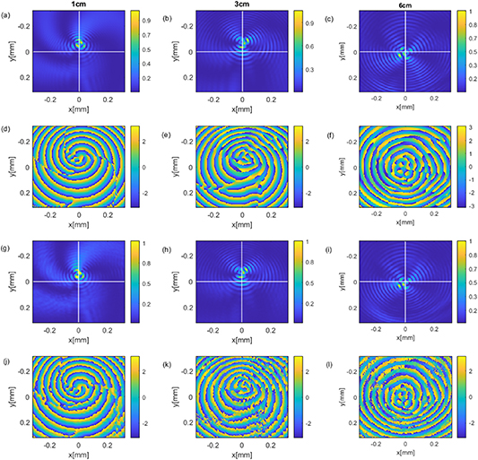
Figure 2. Curving beam with linearly varying OAM at three different locations. The locations are: 1 cm (left column), 3 cm (middle column) 6 cm (right column). Top two rows: simulation results—intensity (in a.u.) (a)–(c) and phase (d)–(f). Bottom two rows: experimental measurements—intensity (in a.u.) (g)–(i) and phase (j)–(l). The white crosshair marks the location of the optical axis.
Download figure:
Standard image High-resolution image
Figure 3. Curving beam with step-wise varying OAM at three different locations. The locations are: 1 cm (left column), 3 cm (middle column) 6 cm (right column). Top two rows: simulation results—intensity (in a.u.) (a)–(c) and phase (d)–(f). Bottom two rows: experimental measurements—intensity (in a.u.) (g)–(i) and phase (j)–(l). The white crosshair marks the location of the optical axis.
Download figure:
Standard image High-resolution image2.3. OAM correlation representation
The OAM correlation representation is given with a correlation function  which is calculated for each OAM value using the following expression:
Here  is the transverse complex amplitude distribution of the analyzed beam. The (x,y) coordinates change through the propagation of the beam, and they are transverse to the z axis as was defined above,
  is the transverse complex amplitude distribution of a beam with the same trajectory propagated to the same distance as
  , with a fixed OAM value specified by the subscript OAM. The range of OAM values was 0–10 with 0.1 increments. s is the area where the intensity of
  is in the range between the maximum intensity and half of it. The integration is performed over s which is unique for each
  . The OAM correlation representation is a measure we use to estimate the local OAM at every propagation distance. It is not a decomposition, as the correlation values are not summed to 1. The results of the OAM correlation representation are shown for the beam with linearly varying OAM in figure 4 and for the beam with step-wise varying OAM in figure 5. In both figures the correlation calculated from the simulation obtained using Fresnel field propagation is shown with blue dots and the correlation calculated from the experimental data is shown with orange dots. The black dotted lines in these figures indicate the designated theoretical values of the OAM. It can be seen that the results derived from experimental data are in good agreement with simulation results and theoretical values.
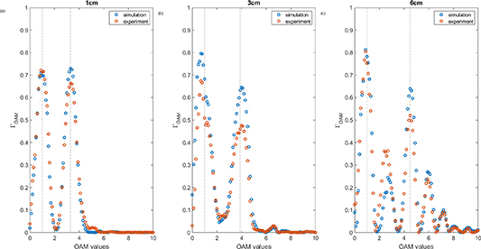
Figure 4. OAM correlation representation for the linearly varying beam at three locations. The locations are: 1 cm (left column), 3 cm (middle column) 6 cm (right column). Shown are both the correlation from the simulation results (blue dots) and from the experimental results (orange dots). The designated values are marked by a black dotted line.
Download figure:
Standard image High-resolution image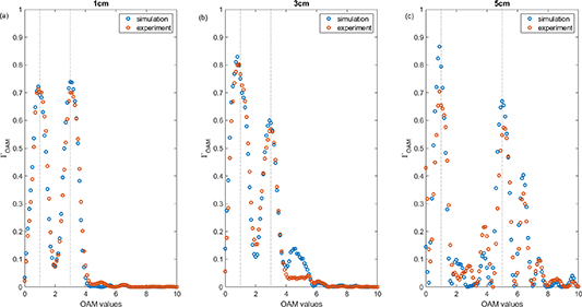
Figure 5. OAM correlation representation for the step-wise varying beam at three locations. The locations are: 1 cm (left column), 3 cm (middle column) 5 cm (right column). Shown are both the correlation from the simulation results (blue dots) and from the experimental results (orange dots). The designated values are marked by a black dotted line.
Download figure:
Standard image High-resolution image
3. Conclusions
We presented a self-accelerating beam with an arbitrary trajectory and a predesigned OAM variation along the propagation direction. A superposition of this beam with another that maintains a fixed value of OAM, generates a complex helical intensity profile that changes its number of strands with propagation. Such a beam constitutes a generalization of the optical Archimedes screw where it accelerates in both its linear momentum and in its angular momentum. We examined this beam experimentally and observed excellent agreement with simulation results and theory. Moreover, we were able to extract the OAM value of each of the beams in different locations along the trajectory following an OAM correlation representation using measurements of the experimental phase and intensity. Our finding could be useful for various applications such as optical manipulation [31], optical communications [35], material processing [37], quantum optics and imaging [38].
Data availability statement
Data underlying the results presented in this paper are not publicly available at this time but may be obtained from the authors upon reasonable request.
Conflict of interest
The authors declare no conflicts of interest.