
Abstract
Structured light refers to the ability to tailor optical patterns in all its degrees of freedom, from conventional 2D transverse patterns to exotic forms of 3D, 4D, and even higher-dimensional modes of light, which break fundamental paradigms and open new and exciting applications for both classical and quantum scenarios. The description of diverse degrees of freedom of light can be based on different interpretations, e.g. rays, waves, and quantum states, that are based on different assumptions and approximations. In particular, recent advances highlighted the exploiting of geometric transformation under general symmetry to reveal the 'hidden' degrees of freedom of light, allowing access to higher dimensional control of light. In this tutorial, I outline the basics of symmetry and geometry to describe light, starting from the basic mathematics and physics of SU(2) symmetry group, and then to the generation of complex states of light, leading to a deeper understanding of structured light with connections between rays and waves, quantum and classical. The recent explosion of related applications are reviewed, including advances in multi-particle optical tweezing, novel forms of topological photonics, high-capacity classical and quantum communications, and many others, that, finally, outline what the future might hold for this rapidly evolving field.
Export citation and abstract BibTeX RIS

Original content from this work may be used under the terms of the Creative Commons Attribution 4.0 license. Any further distribution of this work must maintain attribution to the author(s) and the title of the work, journal citation and DOI.
1. Introduction
There is a saying by Claude Debussy (1862.8.22–1918.3.25), a French impressionist musician, that 'Music is the arithmetic of sounds as optics is the geometry of light.' Indeed, although belonging to very different disciplines, music and optics are inextricably related by the similarity of their physical structures, as unveiled by Debussy. In Debussy's age, rays and geometric optics were still the most prevailing tools to describe light, thus Debussy used the term of 'geometry of light.' While, soon after, wave optics emerged as a new branch of optics to describe light by waves gradually took the upper hand, and it was argued that geometric optics is just a special case of wave optics when the wavelength is approaching zero [1]. As time went on, more branches of optics emanated to unveil deeper physics and general structures of light, such as electromagnetic optics, quantum optics, and recent advances of quantum–classical connection [2–4] (figure 1). Today, the relationship between music and optics can be more deeply understood because more tools have emerged to describe light. For instance, the connection between music and optics can be made explicitly by considering sound and light as waves, as the sound (acoustic wave) and the light (electromagnetic wave) are both waves. Debussy's story inspires people to everlastingly pursue the more general structures of light by toolkits including rays and waves in order to deepen the understanding of the beauty of nature and science.

Figure 1. The schematic diagram of the evolution of branches of optics.
Download figure:
Standard image High-resolution imageIn recent advances of structured light, peoples have been able to control customized structures of light in many degrees-of-freedom (DoFs) such as intensity, phase, polarization, orbital angular momentum (OAM), fuelling fundamental physics and practical applications for both quantum and classical fields [5–9]. While it is still an everlasting topic to push the limit of structured light into higher dimensions and flexibility. The key to address this challenge is to explore the most fundamental symmetry of light, so as to exploit diverse tools to construct on-demand structured light in a better way. In fundamental physics, many kinds of symmetric groups were used to deal with special physical problems [10]. For instance, SU(2) is a general symmetry describing paraxial particle beams, and SO(3) generally describing the particle behavior in central potential fields [10]. Thus, the SU(2) symmetry can provide a basic tool to describe a general set of paraxial light beams, which has been widely applied in optics, such as photon statistics [11–13], beam splitter [14], polarization optics [15–17], and nonlinear wave-packet dynamics [18, 19]. However, the use of SU(2) (symmetry) in the structured light community is still in its adolescence. Thus, it is an advantage to exploit SU(2) mathematics and physics to establish generalized types of structured light for extending its advanced applications.
In this tutorial, the quintessential tools to tailor light, rays, waves, symmetry and geometry, are discussed in a unified and generalized framework. In particular, it demonstrates how to exploit mathematics of SU(2) symmetry to tailor nontrivial geometric pattern and ray-wave coupled structures of light. The theoretical framework especially unveils new field of applied physics such as higher-dimensional mode control and quantum–classical connections. Catering the structured light revolution, I concentrate on new understanding of diverse exotic forms of structured light based on the physics of SU(2) symmetry and geometry, and how this has fueled many exciting applications, appealing to a broad applied physics community and in particular those optical physicists working in multi-disciplinary fields. This tutorial starts from several fundamental questions then toward profound and universal mechanism, the style of which will make it useful to students and emerging researchers, while the comprehensive review nature will make it invaluable to senior researchers in the field too.
The content of this tutorial is arranged as follows. The following section 2 firstly answers the question—what is the universal symmetry to describe light?—the SU(2) symmetry, and provides the clear mathematical basis of SU(2) (symmetry, matrix, group, operation and transformation). Then, I demonstrate how the basic mathematics is used in physics, especially, the quantum linear oscillator, and how the SU(2) coupled linear oscillator theory is used to describe a general family of structured light modes. In section 3, the framework of SU(2) symmetry of light is extended to develop the intriguing classical-quantum coupled theory—ray-wave duality, whereby more diversified structured light beams can be represented as the generalized coherent state superposed by various eigenstates. Such generalized ray-wave structured light has more intriguing properties of OAM frequency-degeneracy, multiple singularities, etc. The further generalization of complex structured light carries on in next sections 4 and 5, including the higher-order ray-wave geometric light corresponding to the generally coupled linear oscillators at 3D spatially orthogonal directions, encompassing exotic Lissajous and trochoidal curve patterns, and the hybrid-order geometric mode as the hybrid superposition of different coherent state wave-packets. In section 6, the methods of experimental generation of various kinds of ray-wave structured light are reviewed, including the at-the-source generation from a laser cavity and the passive modulation by digital holography. In section 7, a graphical representation is given to show that the complex ray-wave geometric light can be elegantly mapped on generalized Poincaré sphere, as an simplified but very versatile model guiding applications. The SU(2) structured light is a general concept, where many other extensions not covered above, we review other exotic SU(2) structured light. In section 9, many potential applications of SU(2) structured light are discussed taking advantage of its unique properties such as ray-wave duality, multiple DoFs, and high-dimensional state. Finally in section 10, we give the perspective of future development of light with general geometric patterns.
2. The general symmetry of light
Symmetry is a basic tool for human being to recognize and classify natural objects. In mathematics, symmetry has more precise definitions and classifications, and is usually used to refer to an object that is invariant under some transformations, including mirror reflection, arbitrary rotation (circular), or rotation of specific angle, and so on. Some examples of objects with different kinds of symmetry in daily life are shown in figure 2. Among which, rotational symmetry (the third column of figure 2) is a phenomenon widely existed in nature, from the movement of galaxies to ocean circulation and typhoon vortices and even to spiral galaxies in the milky way, manifesting themselves not only in macroscopic matter but also in structured electromagnetic and optical fields. In modern mathematics, symmetries are generally defined as invariances under transformations. In the case rotational symmetry, it can be defined as invariance under SU(2) or SO(3) transformation, where SO(3) is the rotation group acting on 3D vectors whereas SU(2) correspond to special unitary transformation on complex 2D vectors, which are very useful to simplify various profound models in particle physics [10]. In fundamental physical courses, SU(2) can be widely seen, which is a general symmetry describing paraxial particle systems such as photon or electron beam, as the SO(3) describing the particle behavior in central potential field, such as the hydrogen atom. Thus, SU(2) provides the basic tool to describe a general set of paraxial light beams.

Figure 2. Selective natural pictures with various kinds of symmetry (mirror symmetry, circular symmetry, and rotational symmetry). The snowflake image comes from https://unsplash.com/photos/rGzUMs-QsCM, other images belong to the author.
Download figure:
Standard image High-resolution imageSU(2) symmetry has been applied in optics in various communities for a long time, such as photon statistics [11–13], beam splitter [14], polarization optics [15–17], and nonlinear wave-packet dynamics [18, 19], to name a few. In the structured light community, SU(2) symmetry is still understudied. Recently, the structured light has attracted growing interest due to its ability to tailor customized distribution of arbitrary DoFs such as intensity, phase, polarization, and OAM [8, 20]. SU(2) transformation has been used in structured light as they are the basis of many transformations and are realized by a large variety of optical elements, and promises to be a useful tool in the exploration of new horizons. Thus, it is an implied advantage to apply SU(2) mathematics and physics to establish more generalized structured light model for extending its applications in more potential dimensions.
2.1. Matrix representation of rotation: SU(2) and SO(3)
Mathematically, a rotation in 2D plane can be represented by a  matrix. If a certain point with coordinate (x, y) is rotated counterclockwise by an α angle around the origin, this process can be represented by a transformation of two-dimensional rotation matrix:
The rotation matrix can be written as the linear combination of two basic matrices, the identity matrix and orthogonal rotation matrix:
Equivalently, the 2D coordinates can be considered as the real and imaginary parts of the complex number, and the rotation matrix can be expressed as the matrix form of the complex number of argument of α, the complex number formation of rotation operation is given by:

corresponding to the transformation form a complex number  to another
  as shown in figure 3(a).

Figure 3. (a) The 2D vector rotation in a complex plane. (b) The 3D vector rotation in a pure quaternion space. (c)–(e) The 3D coordinate rotation transformation based on the three Euler angles.
Download figure:
Standard image High-resolution imageBecause beams of light are actually defined in 3D space, with a longitudinal axis (z) and transverse plane ( ), we will also consider how these 2D rotations can be generalized in 3D. For the 3D rotation, the operation can also be represented by matrix, as well by the quaternion formation (akin to the complex number formation) [21], that
  , where
  . When a = 0, the quaternion only has imaginary parts, namely the pure quaternion
  , which can represents an arbitrary 3D vector
  . Without loss of generality, we consider the rotation axis passing through the origin,
  (
( ,
,  ,
,  ), a 3D vector
  is transformed into
  after rotation by a ϕ angle, as shown in figure 3(b). This transformation can be expressed by the multiplication of quaternion:

where the transformation quaternion is given by:

Therefore, a certain quaternion  can generally represent a rotation transformation in 3D space, the matrix formation of which can be given by [22]:
that can be simplified into a  partitioned matrix and each partitioned part represented by a complex number:
The quaternion is always defined under normalization  , correspondingly, the matrix Q of equation (7) is a unitary matrix, that can be written into argument formation:
In mathematics, the special unitary group SU(2) is the group of  unitary matrices with determinant 1. Thus, equation (8) can be seen as a definition of SU(2) matrix. SU(2) symmetry means the symmetry under SU(2) matrix transformation. The group constructed by the matrix multiply operation is termed as SU(2) group, which is isomorphic to the group of all normalized quaternions transformation, completely describing the 3D fixed-axis rotation and generally revealing the spatial axial rotation symmetry.
SU(2) group completely describes the 3D fixed-axis rotation operation, while the rotation axis can be selected arbitrarily, thus it actually represents general 3D spatial rotation. A well endorsed description of arbitrary 3D rigid body rotation is using Euler angles [23],  , corresponding to three composed elemental rotations [rotations about the three axes through the origin of a coordinate system, see figures 3(c)–(e)], with matrix representations of:
and the general rotation is represented by the multiplicative matrix. In mathematics, 3D rotation group, often denoted SO(3), is the group of all rotations about the origin of  under the operation of composition. Thus, the SO(3) matrix can be defined by:

Three-dimensional real space rotation can be equivalently represented by the SU(2) matrix of a two-dimensional complex plane,

where
This rotation model leads us to the most intuitive approach: while the quaternion and the Euler description can both describe 3D rotations, the Euler description can suffer from singularity issues (Gimbal lock), a problem known in the world of animation, making the quaternion representation advantageous in some cases.
Locally, SU(2) and SO(3) groups are isomorphic, based on equations (10)–(12). SU(2) matrix can be safely used for optics if the possible transformations of optical field are unitary in the general condition.
2.2. SU(2) in physics
2.2.1. SU(2) in classical mechanics.
SU(2) provides a very simplified expression for complex spatial rotation, which has a large number of applications in physics. For instance of the classical mechanics, it is widely used to describe macroscopic and microscopic oscillation phenomena [24–26]. The 2D harmonic oscillation can be expressed as  , where Ax
(Ay
) refer to the amplitude, ω1 (ω2) the frequency of oscillation, φ1 (φ2) the phase factor at x (y) direction. Applying additional rotation motion onto a 2D harmonic oscillation
, where Ax
(Ay
) refer to the amplitude, ω1 (ω2) the frequency of oscillation, φ1 (φ2) the phase factor at x (y) direction. Applying additional rotation motion onto a 2D harmonic oscillation ![$[x_1(t),y_1(t)]$](https://content.cld.iop.org/journals/2040-8986/23/12/124004/revision2/joptac3676ieqn22.gif) , we can realize a periodic trochoidal motion
, we can realize a periodic trochoidal motion ![$[x_2(t),y_2(t)]$](https://content.cld.iop.org/journals/2040-8986/23/12/124004/revision2/joptac3676ieqn23.gif) , this process yields an SU(2) transformation:
, this process yields an SU(2) transformation:
where the oscillation with a trajectory of Lissajous curve is transformed into the oscillation with a trochoidal trajectory, see figure 4 for the example illustration with parameters of  ,
,  ,
,  ,
,  . Summarily, the SU(2) provides a compact mathematical tools to describe more complex group of classical motion modes, i.e. the modes coupled to Lissajous-trochoidal geometric curves.

Figure 4. Schematics of 2D harmonic oscillators: (a) the oscillation is composed by two linear oscillations with frequency ω1 and ω2 along a Lissajous curve; (b) the oscillation is composed by two angular oscillations with frequency ω1 and ω2 along a trochoidal curve.
Download figure:
Standard image High-resolution image2.2.2. SU(2) in quantum mechanics and optics.
In quantum mechanics, the physical quantity is not represented by real functions, e.g. x(t) and y(t), but by operators, e.g.  and
and  (the hat symbol '
  ' will be omitted hereinafter in this article just for the convenience of writing), and the detailed possibility distribution (wavefunction) of corresponding operator is determined by a certain Hamiltonian [27]. For a simple 1D linear oscillator, the Hamiltonian is given by:
where m is the mass, ω is the unperturbed frequency, p is the momentum operator, x is the coordinate operator,  and a are the ladder (creation and annihilation) operators of photon, and
  is the reduced Planck constant. Under coordinate representation, the discrete eigenstates
  (
( ) are solved by Hermite function:
where  , and Hn
represents Hermite polynomials, with corresponding eigenvalues:
, and Hn
represents Hermite polynomials, with corresponding eigenvalues:
Generally, the Hamiltonian for the 3D linear harmonic oscillator is given by:
where  . We take the application in optics for an illustration. The representation of a laser beam often includes transverse and longitudinal modes, which are yielded by the Hamiltonian
  for the 3D transversely symmetric harmonic oscillator in quantum optics [28], where ω0 and ωz
are the frequencies of linear oscillations at transverse and longitudinal directions,
for the 3D transversely symmetric harmonic oscillator in quantum optics [28], where ω0 and ωz
are the frequencies of linear oscillations at transverse and longitudinal directions,  and
and  are the creation and annihilation operators for the photon of transverse mode (
 ) and longitudinal mode (i = z), and
  is the reduced Planck constant. The eigenstates
  (
( ) of the Hamiltonian
  can be generated by the ladder properties of creation operators from the fundamental Gaussian mode as the ground state [28, 29]:
with eigenfrequency of  , where the transverse mode frequency
  and longitudinal mode frequency
  . Eigenstates as described by equation (18) are just corresponding to the well-known Hermite–Gaussian (HG) modes under the Cartesian coordinate representation, with the transverse mode indices of n and m at x- and y-directions respectively, and the longitudinal mode index l at z-direction; and corresponding to Laguerre–Gaussian (LG) modes under the representation of cylindrical coordinate.
Nevertheless, recent advance of structured light unveiled that a laser beam can also harness complex patterns outdoing the transverse symmetry. As such, it should be generally yielded by the Hamiltonian  of separable 3D harmonic oscillator, where ωx
, ωy
, and ωz
are the frequencies of linear oscillations along x-, y-, and z-axes. The separable 3D harmonic oscillator is also called as generalized oscillator, because it can degrade into 3D transversely symmetric harmonic oscillator when
of separable 3D harmonic oscillator, where ωx
, ωy
, and ωz
are the frequencies of linear oscillations along x-, y-, and z-axes. The separable 3D harmonic oscillator is also called as generalized oscillator, because it can degrade into 3D transversely symmetric harmonic oscillator when  . Corresponding to an SU(2) rotation along a fixed axis of the 3D transversely symmetric harmonic oscillator, the general 3D harmonic oscillator can be transformed by transversely symmetric harmonic oscillator via applying SU(2) unitary transformation on ladder operators of transverse oscillators [28, 29]:
Similarly according to the property of ladder operators, the eigenstates of Hamiltonian  are given by:
with eigenfrequency of  , where the transverse mode frequency
  and longitudinal mode frequency
  . Eigenstates in equation (20) are corresponding to the Hermite–Laguerre–Gaussian (HLG) modes [30, 31] with transverse mode indices of (n, m) and longitudinal mode index of l under Cartesian coordinate representation. Of particular note, when ϕ = 0 or
  ,
,  are reduced into HG modes; when
  , LG modes. The evolution of the wavepacket of
  versus θ and ϕ is shown in figure 5. The two angles also refer to mapping angles on generalized Poincaré sphere (see details in section 7).

Figure 5. SU(2) eigenstate of coherent field for representing HLG mode: the wavepacket of  (
( ) versus θ and φ. The plotting is based on the principal in [30] (colormap: darkness to brightness means 0 to 1 for intensity and
  to π for phase).
Download figure:
Standard image High-resolution imageIn order to obtain the analytical expression of terms of equation (20), we exploit the Wigner d-matrix, which is a unitary matrix in an irreducible representation of the SU(2) groups [32]. In terms of the Wigner d-matrix, an eigenstate equation (20) of the Hamiltonia  can be analytically expressed as a linear combination of a set of eigenstates equation (18) of the Hamiltonia:
where the elements of Wigner d-matrix are given by:
Using equations (21) and(22), we can numerically calculate the wave-packet of any mode states of HLG mode.
Hereinbefore, the SU(2) matrix was shown as an effective toolket to describe the transformation for both geometric rays and wave eigenfunctions. In the next section, more complex coherent states exploiting SU(2) symmetry will be introduced to deeper physics of quantum–classical connection and ray-wave duality of light.
3. Rays and waves: from quantum to classical
In this section, a ray-wave duality model for describing a general class of geometric beams is reviewed. Following the the coupled harmonic oscillator model, various HLG eigenmodes can be represented by a general SU(2) transformation, but there are still a large number of structured lights uncovered. Hereinafter, increasingly complex geometric modes with more intriguing properties are demonstrated, as well-defined superpositions of special sets of eigenstates. In which, SU(2) symmetry still play a important role in the generation of various complex quantum coherent state, for representing more intriguing structured light beams with quantum–classical coupled properties.
3.1. Schrödinger coherent state
A coherent state is a specific quantum state whose behavior most closely resembles the classical state, where the quantum probability wave-packet can be coupled with classical movement, which is particularly adapted for studying the quantum-to-classical transition [33–35]. According to the definition of coherent state of Schrödinger's original motivation, i.e. Schrödinger coherent state [36, 37], the coherent state under coordinate representation is given by:
Substituting equations (15) and (16) into equation (23) and applying the generating function of Hermite polynomials,  =
=  , we get:
where δ is the argument of α. Then, the probability wave-packet of Schrödinger coherent state can be derived by:
As shown in figure 6, the peak of wave-packet of is along the trajectory of corresponding classical oscillator, i.e.  , manifesting the quantum–classical coupling. Theoretically, coherent states are always minimize quantum uncertainty, the squeezed states of wave packet with squeezed uncertainty is not included in the discussion of this tutorial.

Figure 6. Schrödinger coherent state. (a) Probability wave-packet of eigenstate of 1D linear oscillator (n = 20). (b) Trajectory of the classical movement of 1D linear oscillator and (c) the probability wave-packet of coherent state (α = 1, ω = 1, δ = 0).
Download figure:
Standard image High-resolution image3.2. SU(2) coherent state
In quantum optics, the Hamiltonian for the 3D linear harmonic oscillator is given by equation (17). Here,  is used to represent the Hamiltonian of conventional transversely symmetric harmonic oscillator, and
  to represent the generalized Hamiltonian after SU(2) transformation. The generalized Hamiltonian of the SU(2)-coupled oscillator can be expanded as:
where  is the Hamiltonian for the 2D isotropic oscillator deciding the transverse wave-packet on (x, y) plane. Figure 7 shows examples for the eigenstate wave-packet, classical trajectory, and coherent wave-packet in this case. The coupling parameters
  are assumed to be real constants, and the operators under Schwinger representation reveal the SU(2)-Lie group accommodating two linear oscillators and an angular momentum oscillator [13, 38]:
Operators Jj
satisfy the SU(2)-Lie commutator algebra ![$[J_i,J_j] = {i}\varepsilon_{i,j,k}J_k$](https://content.cld.iop.org/journals/2040-8986/23/12/124004/revision2/joptac3676ieqn69.gif) (
( ), where the Levi-Civita tensor
  is equal to +1 and −1 for even and odd permutations of its indices, respectively, and zero otherwise. The Hamiltonian in equation (26) can not only represent a host of entanglement mechanisms [39, 40] but also be associated with astigmatism and aberration in wave optics, relevant in high-order laser pattern formations [28, 41]. For the statistics of quantum number at transverse oscillation, SU(2) coherent state is defined as [18, 19]:

where  are the ladder (creation and annihilation) operators of angular momentum, and j is a certain integer or half-integer that represents angular-momentum quantum number. Using the disentangling theorem for angular-momentum operators, we can rewrite equation (28) in the following equivalent form [13]:
where τ is an arbitrary complex number. Hereinafter, we express equation (29) into eigenstates representation via unitary transformation. According to Taylor expansion, the exponential operator in equation (29) can be expanded as:
Substitute equation (30) into equation (29) and apply unitary transformation into angular-momentum representation:
According to the property of ladder operators:

Equation (31) can be rewritten as:
After substituting  and
and  (N is a constant integer, K is integer yielded
  ), we get:
where the states  mean the states with K bosons in the first mode and
  bosons in the second mode, sometimes also noted as
  . In another usually used form, τ is rewritten as the normalized argument form
  , and equation (34) can be rewritten as the phase state:
where the eigenstates  should fulfill the orthogonality
  , where
  is the Kronecker delta, and the completeness
  ,
,  ,
,  .
.
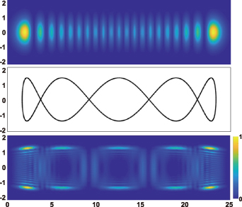
Figure 7. SU(2) coherent state. (a) Probability wave-packet of eigenstate of 1D linear oscillator (n = 20). (b) Trajectory of the classical movement of 1D linear oscillator and (c) the probability wave-packet of coherent state (α = 1, ω = 1, δ = 0).
Download figure:
Standard image High-resolution image3.3. Frequency-degenerate state
In order to realize SU(2) coherent state in a laser cavity, the eigenstates should be the eigenmodes of the resonator and fulfil the coherent-superposition condition of SU(2) wave-packet [35, 42]. Without loss of generality, we consider a plano-concave cavity with the length of L, formed by a gain medium, a concave spherical mirror with the radius of curvature of R as the output coupler, and a plane mirror high-reflective for laser. The eigenmodes  (
( are the indices of transverse mode and l is the index of longitudinal mode) and the eigenvalues
  for a laser cavity can be solved from the Helmholtz equation:

Under the paraxial approximation, the eigenmodes that are separable in Cartesian coordinate can be expressed as HG modes:
where  is the Gouy phase,
  represents the Hermite polynomials of nth order,
  ,
,  is the eigenmode frequency, c is the speed of light,
 ![$\widetilde{z} = z+(x^2+y^2)z/[2(z^2+z_R^2)]$](https://content.cld.iop.org/journals/2040-8986/23/12/124004/revision2/joptac3676ieqn99.gif) ,
,  ,
,  is the beam radius parameter, and λ is the emission wavelength. The eigenmode frequency of resonator is given by [42, 43]:
where the longitudinal mode spacing  , here the minor disparity between the physical length and the geometric length is neglected. Without consideration of symmetry breaking, the transverse mode spacing should be
  . The mode-spacing ratio
  reveals the degeneracy, which is varied in the range between 0 and 1/2 by changing the cavity length as
  . The frequency difference in the neighborhood of the indices
  is given by
  , which can illustrate the various degeneracy states distribution as topological joints in the fractal spectrum [43]. Figure 8 depicts a diagram of the frequency-degenerate spectrum, where some degeneracy states
  are marked at corresponding positions. In order to fulfill the condition of coherent superposition, the frequency of every decomposed eigenmodes should be a constant, which requires a coupling effect between transverse and longitudinal modes. If the transverse mode at x-axis and longitudinal mode are coupled, i.e.
  , we can choose a frequency-degenerate family of HG modes as the complete set of orthogonal bases:

where n0, m0, and l0 are constants with  , thus the constant frequency should be:
which meets the required form of transverse mode locking [44–47], and the corresponding laser wave-packet of SU(2) coherent state is given by:
sharing the same form of equation (35). Here we have already proved that frequency-degenerate state of laser cavity fulfills the condition for generating a laser wave-packet as SU(2) coherent state.

Figure 8. Frequency-degenerate spectrum and the ray representation in laser cavity. The frequency-degenerate spectrum  of the ideal spherical cavity as a function of the normalized cavity length
  for the range of
  ,
,  , and
, and  , where some degeneracy states
  are marked at corresponding positions with corresponding schematics of ray representation of SU(2) oscillation.
Download figure:
Standard image High-resolution imageWe can also use Laguerre–Gaussian (LG) modes being separable in circular coordinate as the eigenmodes to generate SU(2) vortex beams:
where the LG modes are given by:
where  ,
,  , and
, and  represents the associated Laguerre polynomial with radial and azimuthal indices of ρ and
  . For
. For  , figure 10 shows the 3D simulation of SU(2) vortex beams with positive, negative, and superposed OAMs, and the inserts show the topological phases of the SU(2) vortex beams. For
  , the SU(2) beams manifest the multi-LG vortex beams [48, 49], where the main OAM at the center is decided by the index n0 and the sub-OAM carried by sub-LG beams is decided by the index m0. To constitute a completed oscillation in cavity, the positive and negative oscillations should be superposed together forming a standing wave mode, the phase state expression of which is
  [35]. Figure 9 shows the ray presentation (a) intensity wave-packet (b)–(d) of intracavity geometric modes versus the coherent state phase. From larger n0 to smaller one, the wave-packets perform from ray-like cases to wave-like cases. Figure 10 shows the transverse patterns of planar and vortex geometric modes and the topological phase of vortex geometric modes at SU(2) coherent state
  with parameters as
  , N = 20, and various n0 and m0. Some cases perform multi-spot shape while some wave fringes unravel the interference among lights on the sub-orbits, which is manifested by the property of ray-wave duality.

Figure 9. Phase states of SU(2) oscillation with ray-wave duality. Intracavity planar SU(2) geometric mode  oscillating at (x, z)-plane at degenerate state
  : (a) the ray representations and (b)–(d) intensity wave-packets with n0 from larger to smaller (
 ) for various φ. The patterns of wave representations from (b) to (d) change from the case of more ray-like properties to that of more wave-like properties.
Download figure:
Standard image High-resolution image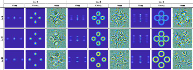
Figure 10. Planar and vortex SU(2) geometric modes. The theoretical intensity transverse patterns of planar and vortex geometric modes and the topological phase of vortex geometric modes at SU(2) coherent state  with parameters as
  , M = 20, and various n0 and m0.
Download figure:
Standard image High-resolution imageThere are also other ways to realize frequency degeneracy in order to fulfill the coherent superposition of SU(2) wave-packet. For instance:

where the integers p and q yield  (κ = 1 selected here, the case of κ ≠ 1 will be discussed in section 6.1 since it is caused by astigmatism), thus the eigenmodes also constitute a frequency-degenerate family with frequency
  . Using the more general equation (44) as the bases of SU(2) coherent state, we can obtain more exotic structured light beams [28, 43].
3.4. Ray-wave duality
Ray-wave duality, as its name implies, describes the effect that a wavepacket behaves matching a prescribed ray families [50, 51]. In this section, it is demonstrated that the ray-wave duality is also the salient property of the geometric mode in degenerate cavity. When an optical resonator is operating close to a frequency-degenerate state, its laser mode and intensity would undergo dramatic changes with the principle that laser modes have a preference to be localized on the periodic ray trajectories under selective gain control, which was called the ray-wave duality or ray-wave correspondence [35, 42, 52, 53]. Like the Schrödinger coherent state coupled with the trajectory of classical oscillator, the SU(2) coherent state can also be coupled with the periodic oscillating trajectories in frequency-degenerate cavity, interpreting the ray-wave duality mode.
Based on geometrical optics, the ABCD matrix is used to characterize the propagation property of the optical ray trajectories inside a stable plano-concave cavity [54–56]. Since the cavity length satisfies  under degeneracy state
  , the corresponding ABCD matrix of the frequency-degenerate cavity is given by:
After n times of round trips in the frequency-degenerate cavity, the matrix is derived as:
Because  is an integer, we have
  ,
,  , and Qth power of A is an unit matrix:
Equation (47) reveals that an optical ray oscillating at an arbitrary position within the cavity would coincide exactly with the initial state after Q times of round trips. Therefore, it is proved that the lasing modes have a preference to be localized on the periodic ray trajectories in a frequency-degenerate cavity. The schematics of classical oscillating trajectories at various states  are shown in figure 8. Manifested by the ray matrix, the parametric equation for each periodic orbit in SU(2) oscillation can be derived [57]. For the planar geometric modes, the orbits can be derived as:
where  is the running index for the different rays, φx
is the phase factor related to the initial position and direction, and + and − in the symbol of ± indicate the backward and forward rays, respectively. Defining the dimensionless variable
is the running index for the different rays, φx
is the phase factor related to the initial position and direction, and + and − in the symbol of ± indicate the backward and forward rays, respectively. Defining the dimensionless variable  , the expression for the ray equation can be expressed as
 ![$\widetilde{x}(z) = \operatorname{Re}[\sqrt{2}{u}_{s}^{\pm }(z)]$](https://content.cld.iop.org/journals/2040-8986/23/12/124004/revision2/joptac3676ieqn135.gif) with:
with:

when  (
( ), the forward and backward rays would be coincidently overlapped, and the bouncing orbits with positive and negative transverse directions share the same location. In this case, the trajectories in frequency-degenerate cavities at various degenerate states
  are depicted in figure 8. For the general spatial geometric mode, the ray equations for the 3D periodic orbits can be written as:
where the dimensionless variable in the y-direction is similarly defined as  with the ray equation
 ![$\widetilde{y}(z) = \operatorname{Re}[\sqrt{2}{v}_{s}^{\pm }(z)]$](https://content.cld.iop.org/journals/2040-8986/23/12/124004/revision2/joptac3676ieqn140.gif) . Here + and − in the symbol of ± indicate the positive and negative OAM states
. Here + and − in the symbol of ± indicate the positive and negative OAM states  , they together constitute a completed oscillation in cavity. For constituting a completed oscillation with both OAM states in a cavity, the phase factors yield
  .
.
The above is the ray representation of geometric modes in frequency-degenerate cavity. Hereinafter, we derive the wave representation coupled with the geometric modes and prove that it fulfills the SU(2) coherent state. In terms of Schrödinger coherent state, the Gaussian wave packet with the central peak moving along the path  can be derived as [57]:
where coefficients  , where
  is the Poisson distribution,
  is the wavefunction of Schrödinger coherent state and
  is the HG function. The wave representation of a Gaussian wave packet moving along the sth ray, equation (50), in a spatial geometric mode can be given by [57]:

where  represents the fundamental mode Gaussian beam and
  the Cartesian coordinates. In terms of equation (52), the resonant mode for the forward and backward components of a complete period is given by [57]:
where the phase term  is associated with the transverse frequency. For
  or
or  , equation (53) represents the planar geometric modes with ray structure on (x, z) or (y, z) plane; for
  , circular vortex geometric modes; for
  and Nx
and Ny
are nonzero, elliptical vortex geometric modes. In the above description, Nx
or Ny
should be large enough to stimulate more ray-like properties, otherwise the pattern will be nearly a certain eigenmode. Hereinafter, we demonstrate the wave representation fulfills the form of SU(2) coherent state. Using planar trajectory (
and Nx
and Ny
are nonzero, elliptical vortex geometric modes. In the above description, Nx
or Ny
should be large enough to stimulate more ray-like properties, otherwise the pattern will be nearly a certain eigenmode. Hereinafter, we demonstrate the wave representation fulfills the form of SU(2) coherent state. Using planar trajectory ( ) for convenience, it can be obtained that
  and
and  , and the planar geometric mode is given by:
Substituting equation (51) into equation (54) and ignoring the constant coefficient, we get:
where the indices of HG modes should also fulfill the frequency-degenerate condition. Setting  , the last term in the external summation notation of equation (55) can be written as:
When  (
( ),
),  and equation (56) is equal to a constant Q; when
  , equation (56) is always a sum of the complex numbers uniformly distributed on the unit circle of the complex plane, thus it should be zero. And then, we use the Dirac notation to represent the spatial mode, and note the set of frequency-degenerate HG modes with number of M as
  , equation (55) can thus be simplified as:
where the coherent state phase  , and the Poisson distribution
  is approximated by Binomial distribution
  when
when  is large enough, where
  is Binomial distribution, according to the central-limit theorem. Then the laser mode equation (57) shares the same form of SU(2) coherent state as equation (35).
Therefore, the SU(2) wave-packet in frequency-degenerate cavity has the property of ray-wave duality, the laser mode can be not only characterized by the wave function representation but also coupled with classical oscillating trajectory given by ray representation. The preponderance of wave-like or ray-like property can be actually controlled by the parameters in SU(2) wave-packet. It is also worth to note that the ray-wave duality effect discussed above originates from laser cavity optomechanism, it is also available to study the ray-wave duality in general freespace electromagnetic fields [50, 58, 59], which should have more flexible applicability beyond the limit of laser cavity condition.
4. Higher-order geometric patterns of light
Based on the theoretical bases introduced in last section, the structured light wave-packet of SU(2) coherent state can be written as the ket formation:
As a salient property of ray-wave duality, the probability wave packet is coupled with the classical movement. Therefore, the wave-packet of the SU(2) coherent state should be located on the corresponding SU(2) geometric trajectory. The trajectory of classical movement of the SU(2) coupled oscillator is yielded by [28]:
where  represents the 3D classical trajectory of the oscillator corresponding to Hamiltonian
  . This SU(2) transformation of classical trajectory equation (59) is coupled with that of operator transformation equation (19), and the coherent state wave-packet of Hamiltonian
  should be located along the trajectory of
  , namely the property of quantum–classical connection. The analytical expression of
  can be solved by [60, 61]:
where the integer  is the running index for the cluster of rays,
  and
and  are the intensities and initial phases of oscillator components at x- and y-axis,
  is Gaussian beam waist parameter, and
  is Gouy phase where zR
is Rayleigh range. Nx
and Ny
are positively correlated with n and m, and
is Gouy phase where zR
is Rayleigh range. Nx
and Ny
are positively correlated with n and m, and  is related to φ in coherent state.
Hereinafter we demonstrate how a higher-order geometric mode is reduced into a HLG eigenmode. The relationship is demonstrated in the first row of figure 11. The selected modes on the poles are shown in the second row of figure 11, that on the interposed regions between the poles and the equator the third row of figure 11, and that on the equators the fourth row of figure 11. Using SU(2) transformation, the modes together with the corresponding classical trajectories in the first row can be transformed into that in the second and third row, vice versa.
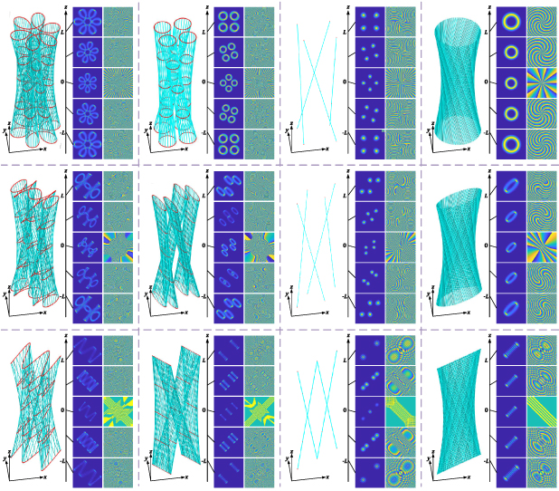
Figure 11. The first column shows the Lissajous-to-trochoidal parametric surface modes, the second column multi-axis HLG modes, the third column planar-to-vortex multi-path geometric modes, and the fourth column eigenstate modes. The first to third rows are corresponding to three different SU(2) angular parameters of  ,
,  , and
, and  .
.
Download figure:
Standard image High-resolution image4.1. Lissajous-to-trochoidal parametric surface mode
For a general case that the ratio of transverse and longitudinal frequency spacings can be expressed as  where (P, Q) is a pair of coprime integers, the ratios of
  and
and  are two rational numbers that can be expressed by:
where  is a pair of coprime integers satisfying
  , the classical trajectory equation (60) is reduced into a ray cluster with limited rays [60, 61]:
which is a ray cluster with QM2 rays, where the meaningful range of k should be  , because Q is the overlapping period for the running of k, P = 1 selected commonly. The representation for SU(2) geometric beams needs to be discussed in frame of Schrödinger coherent state, which could be referred in [57]. The trajectory
  represents a ray cluster including QM2 rays uniformly distributed on a Lissajous parametric surface, which is also a kind of ruled surface. At a certain transverse plane, the transverse pattern of the ray cluster illustrates multiple dots uniformly distributed on a certain Lissajous curve. The corresponding general ray cluster
  after SU(2) transformation includes the QM2 rays uniformly distributed on a trochoidal parametric surface. At a certain transverse plane, the transverse pattern illustrates the structure of multiple dots distributed on a certain trochoid (at the poles of PS), or a Lissajous curve (at the equator of PS), or the topological curve interposed between Lissajous curve and trochoid. The corresponding coherent state equation (58) generally harnesses the wave-packet located on the 3D Lissajous-to-trochoidal parametric surface (trochoidal parametric surface at the poles of PS and Lissajous parametric surface at the equator of PS). The SU(2) PS and some represented Lissajous-to-trochoidal parametric surface modes with corresponding classical trajectories are shown in the first column of figure 11.
4.2. Multi-axis Hermite–Laguerre–Gaussian mode
For a special case of  , i.e. q = 0, we can get
  , also get
  based on the frequency-degenerate condition, then it can be deduced that p = Q, q = 0, and
  here, thus
  and the classical trajectory equation (63) is reduced into:
which is a spatial ray cluster with QM2 rays, but the dots distribution is no longer along a Lissajous curve but reduced to compose multiple linear oscillation orbits in a certain transverse plane. The general SU(2) trajectory  shows multip-axis elliptical orbits distributed on subset uniparted hyperboloid ruled surfaces, where the axes are located on a main uniparted hyperboloid ruled surface, composing a SU(2) symmetric structure. The corresponding coherent state wave-packet equation (58) is reduced into:

which refers to multi-axis vortex beams, also named as multi-axis HLG modes. The subset multiple HLG modes propagating along the Q axes uniformly distributed on the main uniparted hyperboloid ruled surface. Specially, the topological charge of a HLG sub-mode vortex is equal to m in the multi-axis HLG mode, the center topological charge of the main vortex is equal to n, and that for the partial phase singularities is QN. The SU(2) PS and some represented multi-axis HLG modes with corresponding classical trajectories are shown in the second column of figure 11.
4.3. Planar-to-vortex multi-path geometric mode
For an even special case of  and
and  , naturally
  ,
,  , and
, and  , the classical trajectory equation (64) is further reduced as:
where the meaningful range of k should be  , which is cluster of Q rays in a planar hyperbola region. The corresponding general trajectory
  after SU(2) transformation is actually the Q rays uniformly distributed on a unparted hyperboloid ruled surface. At a certain transverse plane, the pattern illustrates multiple dots uniformly distributed on a ellipse orbit. The corresponding coherent state wave-packet is reduced from equation (65) into:
which harnesses a multi-path geometric mode with the Q paths uniformly distributed on the main uniparted hyperboloid ruled surface, which can be obtained by replacing the sub-HLG beams in the multi-axis HLG mode into fundamental Gaussian beams. With the SU(2) transformation, the planar multi-path geometric mode is transformed into vortex multi-path geometric mode. Specially, the topological charge of the center vortex is equal to n, and that for the partial phase singularities is QN. The SU(2) PS and some represented planar-to-vortex multi-path geometric modes with corresponding classical trajectories are shown in the third column of figure 11.
4.4. From coherent state to eigenstate
For a even further special case when  , the ratio of
  is approaching a irrational number. There would be infinity classical rays in trajectory equation (66) covering the whole inside region of a hyperbola, and the corresponding coherent state is reduced into an eigenstate HG mode. After the SU(2) transformation, the rays in trajectory
  would cover the whole surface of an uniparted hyperboloid, and the corresponding coherent state is reduced into an eigenstate HLG or LG vortex mode (
 ). This process subtly reveals the nature of photons traveling along straight lines in the formation of various basic vortex modes. The OAM PS and some represented HLG modes with corresponding classical trajectories are shown in the fourth column of figure 11. It is also a condition of N = 0 that the coherent state is naturally reduced into an eigenstate, where there is only one component state in the coherent state wave-packet.
5. Hybrid-order and vectorial structured light
In contrast to conventional beams, a geometric mode opens new DoFs to describe its structures taking advantage of the ray-wave duality, such as ray numbers, frequency-degenerate ratios, and coherent phase. In this section, the further generalized models for geometric light are discussed, opening even more DoFs to tailor geometry of light.
5.1. Hybrid-order SU(2) geometric mode
Any SU(2) geometric beam discussed in prior section is coupled with a periodic ray trajectory. Is it possible to exist generalized cases of geometric modes that can be coupled with multiple ray trajectories? Recent works demonstrate that two and more SU(2) geometric mode sharing a coincident projection at the highly reflective mirror plane can coexist in a single cavity [62]. Such modes, namely hybrid-order SU(2) geometric modes, can be generated by forcing the laser to oscillate on two different trajectories with orthogonal transverse orders and coherent-state phases simultaneously, each one has a different transverse orders Ni
( ) in equation (41). A hybrid SU(2) geometric mode with two components can be described as:

where  represents the degenerate state, φ is coherent-state phase and
  represents phase state, the trajectory shape is determined by Ω and φ, the trajectory scale is determined by transverse orders Ni
, the lager Ni
corresponds to the outer trajectory and the smaller one corresponds to the inner trajectory,
represents phase state, the trajectory shape is determined by Ω and φ, the trajectory scale is determined by transverse orders Ni
, the lager Ni
corresponds to the outer trajectory and the smaller one corresponds to the inner trajectory,  represents a SU(2) geometric mode with parameters
  determined by equation (58), such compact notations reveals multi-DoFs entanglement. To fulfill the coincident project condition, transverse orders N, which is directly proportional to pump off-axis displacement, and satisfies a mathematical relation to ensure at least one shared coincident projection points as [62]:
When solving this equation, we need to first consider the value of integer Q. The lowest possible Q is 5, because no shared coincident projection can be found for  . For Q = 6, there is also a simple solution, that is depicted in figures 12(a) and (b). For higher values of Q, things become complex, we can divide the possible situation into 4 cases. Figure 13 shows the trajectory combination cases for Q = 7, Q = 8, Q = 9, and Q = 10, respectively. Importantly, in contrast to pure SU(2) geometric modes, the hybrid geometric mode opens new DoF to distinguish geometry of light—the combinatorial number C, which refers to how many cases of available superpositions of hybrid ray trajectories:
-
 The number of inflection points is n − 2 for (chiral, non-axisymmetrical) and n for (achiral, axisymmetrical), respectively. For half-plane , it is for and for so that the combinatorial number is .
 -
The number of inflection points is n for both and . For half-plane , it is for both and so that the combinatorial number is .
-
The number of inflection points is n − 1 for both and . For half-plane , it is for both and so that the combinatorial number is .
-
The number of inflection points is n for bothand , respectively. For half-plane , it is for and for so that the combinatorial number is .


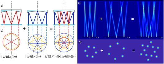
Figure 12. Generation of hybrid SU(2) geometric modes. Example of  (a) intra-cavity classical trajectory with (b) corresponding auxiliary circles. (c) Planer mode wave-packet and (d) vertex mode (
 cross-section) Auxiliary circle describes the parametric function of the planer trajectory in equation (64).
Download figure:
Standard image High-resolution image
Figure 13. Complicated hybrid SU(2) geometric modes with multiple trajectory-combination numbers and multi-trajectory superposition. The solutions are represented in auxiliary circle form.
Download figure:
Standard image High-resolution imageFor a hybrid trajectory with same parameters of Ω, Ni
, and φ, the geometry can still be diverse with different value of C. Similar to pure SU(2) geometric modes, the hybrid SU(2) geometric modes can also be converted into vortex geometric modes carrying OAM with astigmatic converter outside the cavity, see example in figures 12(c) and (d). Unlike planar SU(2) geometric modes, the evolution of phase state for vortex geometric modes just corresponds to the axial rotation (also the rotation of auxiliary circle) of
  according to SU(2) rotational symmetry. As a result, the two eigenstate components do not intersect like planar modes. However, on any lateral propagation plane forms the equilateral star shapes, where the angle difference between inner and outer shape is
  .
.
5.2. Hybrid-order SU(2) vector beam
According to the principle of hybrid trajectory in last section, the general representation of hybrid SU(2) geometric vector mode can be given by introducing polarization as another DoF:

where transverse order states  and
and  of the two components fulfill the condition for sharing a coincident projection of inflection points, which are also corresponding to the OAM state
  and
and  ; phase states
  and
and  manifest that the two components have opposite classical trajectories; the horizontal and vertical linear polarized states
  and
and  can be replaced by other pairs of orthogonal polarized states. In terms of the theories of ray-wave duality, the analytical expression for the hybrid SU(2) VBs can be given by:
where J1 and J2 are the Jones vectors representing two orthogonal polarizations. For Nx
or  , equation (71) represents the planar hybrid SU(2) VBs with geometric structure on the (x, z) or (y, z) plane; for
  , the OAM hybrid SU(2) vector vortex beams; for
  , the general elliptical hybrid SU(2) vector vortex beams. When an SU(2) vector beam is controlled into ray-like state with large enough Nx
and Ny
without interference among light on sub-orbits, the wavefunction along different orbits are independent for calculating the intensity:
, the general elliptical hybrid SU(2) vector vortex beams. When an SU(2) vector beam is controlled into ray-like state with large enough Nx
and Ny
without interference among light on sub-orbits, the wavefunction along different orbits are independent for calculating the intensity:
where  is the Frobenius norm of vector Ψ.
In contrast to the scalar hybrid-order geometric beams, the hybrid vector beams can have more interesting vectorial properties, different intensity patterns can be obtained after projection to different polarization state, as shown in figures 14(a) and (b). A scalar hybrid beam always show the star shape pattern (figure 14(a1)), while a vector hybrid beam can show both star shape and polygonal shape under different polarization projections (figure 14(b1)). Moreover, the hybrid-order scalar beams and vector beams have very different topological phase. For the scalar hybrid beam, its phase difference of two orthogonal polarized components shows a multi-singularity vortex pattern (figure 14(a2)), while the vector hybrid beam shows the phase distribution of a multi-singularity flower pattern (figure 14(b2)).

Figure 14. Experimental results of Intensity patterns, vectorial properties (left), and theoretical phase distributions (right) of various kinds of general SU(2) vector beams: (a)  , (b)
, (b)  , (c)
, (c)  , and (d)
  .
.
Download figure:
Standard image High-resolution image5.3. General SU(2) vector beams
Using general digital modulation technique onto geometric beams, a normal SU(2) geometric beam can be modulated as a general SU(2) vector beam, where arbitrary amplitude, phase, and polarization for each orbit can be modulated. By modifying equation (53), a general SU(2) vector beam can be given by:
where we set  for convenience; As
, φs
, and Js
are the amplitude, phase, and polarization Jones vector of light at the sth orbit.
for convenience; As
, φs
, and Js
are the amplitude, phase, and polarization Jones vector of light at the sth orbit.
When an SU(2) vector beam was controlled into ray-like state with large enough Nx and Ny without interference among lights on sub-orbits, the wavefunction along different orbits are independent without interference to each other. Thus, intensity pattern can be simplified as:
where  is the Frobenius norm of vector
  . Hereinafter, we derive the expression for the polarization projection states. The Jones matrix for a linear polarizer with a inclined angle of θP
is
. Hereinafter, we derive the expression for the polarization projection states. The Jones matrix for a linear polarizer with a inclined angle of θP
is ![${{\mathbf{J}}_{P}} = \left[ \begin{matrix} \cos {{\theta }_{P}} & 0 \\ 0 & \sin {{\theta }_{P}} \\ \end{matrix} \right]$](https://content.cld.iop.org/journals/2040-8986/23/12/124004/revision2/joptac3676ieqn272.gif) , which can project the light into the linear polarization state with inclined angle of θP
. The SU(2) geometric vector beam after projection can be given by:
, which can project the light into the linear polarization state with inclined angle of θP
. The SU(2) geometric vector beam after projection can be given by:
When Nx and Ny are both large enough, the lights on various orbits cannot make interference to each other, the intensity pattern can be given by:
Figures 14(c) and (d) show the intensity patterns after polarization projection and topological phase distribution of two general SU(2) vector beams as intermediate states between pure scalar hybrid beams and maximally nonseparable hybrid vector beams. Their phase distributions show interesting polygonal shapes but with divide of non-singularity and multi-singularity regions.
6. Generation of geometric modes of light
In this section, we systematically review the methods to generate various kinds of SU(2) structured light, including the conventional laser cavity control and the recently advanced digital holographic shaping methods. In addition, here we not only describe the technical approaches, but also provide strict theoretical background to explain why and how the corresponding approaches can control the on-demand SU(2) structures.
6.1. Laser generation of SU(2) geometric beam
From the theories in above sections, the coupling between transverse and longitudinal modes plays a crucial role in manipulation of SU(2) structures in a laser beam. Thus a direct way to realize it is using the solid-state laser cavity with precise geometric control. For exploring the structured light fulfilling a set of paraxial multi-pass ray paths, the confocal cavity with special control of frequency-degenerate transverse and longitudinal modes is endorsed as the effective tool, which is firstly proposed by Herriott et al for a long history [63]. Such frequency-degenerate resonator scheme was also usually called as Herriott-type cell or Herriott-type cavity [64–66]. In recent decade, the Herriott-type cavity was used as laser oscillator with gain control of off-axis pumping to selectively generate SU(2) geometric beam [35, 42, 67]. In section 3.3, we have demonstrated that the frequency-degenerate cavity can fulfill the condition of generating SU(2) wave-packet. However, it is still a question: how to excite such mode in a frequency-degenerate cavity? In this section we give a proof that using off-axis pumping onto the degenerate cavity can excite the output laser mode as the form of SU(2) wave-packet.
To theoretically prove this, considering the gain distribution  in a cavity, the resonant modes of the laser system pumped by a localized source can be solved from the inhomogeneous Helmholtz equation [42]:

where  ,
,  is the given wave number of the laser with given wavelength λ0, the factor ηc
represents the conversion efficiency for the excitation source, and α is a small loss parameter including losses from the scattering, the absorption, and the output coupling. If we set the gain distribution
is the given wave number of the laser with given wavelength λ0, the factor ηc
represents the conversion efficiency for the excitation source, and α is a small loss parameter including losses from the scattering, the absorption, and the output coupling. If we set the gain distribution  as the off-axis pumping spot distribution, we can solve the corresponding wave packet expression. And then if we set the cavity length L in the boundary condition as that of a frequency-degenerate state,
  , we can prove the wave packet result fulfills the SU(2) coherent state, as the form of multi-path geometric mode. The process can be expressed as the following:
We arrange the complete theoretical derivation from inhomogeneous Helmholtz equation to SU(2) coherent state in supplementary materials (available online at stacks.iop.org/JOPT/23/124004/mmedia) in details. In conclusion, the frequency-degenerate cavity with off-axis pumping can emit the multi-path geometric laser mode of SU(2) coherent state.
6.2. Laser generation of higher-order SU(2) geometric beam
For generating higher-order SU(2) geometric beams from a laser, the technique exploits the astigmatism in normal frequency-degenerate cavity, namely degenerate astigmatic cavities [69, 70]. This case is for the more general mode coupling at transverse directions, that  , the transverse symmetry breaking occurs and more frequency degeneracies arise, and the effective cavity lengths in x-axis and y-axis can be expressed as
  and
and  , where d is the small difference between Lx
and Ly
(
, where d is the small difference between Lx
and Ly
( ), and result into different transverse mode frequencies at two orthogonal directions of
  and
and  , which correspond to the frequencies of separable 3D harmonic oscillator in equation (17). The small difference d between the two equivalent astigmatic cavity lengths, Lx
and Ly
, can be realized by applying an anisotropic crystal in experiment. The pump light spot also needs to be tuned as larger shape to accommodate higher-order transverse modes. In order to describe the more detailed frequency degeneracy in the cavity of transverse symmetry breaking, we introduce a dimensionless parameter ξ to reveal the fine adjustment on the cavity length as
, which correspond to the frequencies of separable 3D harmonic oscillator in equation (17). The small difference d between the two equivalent astigmatic cavity lengths, Lx
and Ly
, can be realized by applying an anisotropic crystal in experiment. The pump light spot also needs to be tuned as larger shape to accommodate higher-order transverse modes. In order to describe the more detailed frequency degeneracy in the cavity of transverse symmetry breaking, we introduce a dimensionless parameter ξ to reveal the fine adjustment on the cavity length as  , where
  , i.e. the effective cavity lengths are given by [43]:
In this symmetry breaking cavity, the transverse frequencies near cavity length  can be derived as:
Applying Taylor expansion of ![${{\sin }^{-1}}\left[ a\left( 1-x \right) \right] = \sum\limits_{n = 0}^{\infty }{\frac{{{f}^{(n)}}(0)}{n!}{{x}^{n}}} = {{\sin }^{-1}}\left( a \right)+\frac{a}{\sqrt{1-{{a}^{2}}}}x+o\left( {{x}^{2}} \right)$](https://content.cld.iop.org/journals/2040-8986/23/12/124004/revision2/joptac3676ieqn287.gif) , we can simplify the equations (81) and (82) as:
, we can simplify the equations (81) and (82) as:

where ![$\beta = d/[\pi R \cos(\pi P/Q)]$](https://content.cld.iop.org/journals/2040-8986/23/12/124004/revision2/joptac3676ieqn288.gif) . An equivalent expressions for the expressions of transverse frequencies transverse frequencies are
. An equivalent expressions for the expressions of transverse frequencies transverse frequencies are  and
and  , based on
  ,
,  , and
, and  . Equations (81) and (82) are the generalized cases of equations (61) and (62) in actual cavity. Substituting equations (81) and (82) into the eigenfrequency equation (38) and using the index notations of
  ,
,  ,
,  , and the frequency difference spectrum near
  can be derived as:
The frequency-degenerate state requires  , thus triple integers
  should fulfill
  to reveal the independence of term
  decided by the main cavity length
  , and the rest terms in equation (85) are written as:
thus the frequency-degenerate states occur at the effective cavity lengths with  .
.
The detailed frequency difference spectrum versus ξ near the cavity length  is shown in figure 15(b), where the frequency-degenerate states occur at corresponding values of
  are selectively marked. For example, under frequency-degenerate condition
  corresponds to
  respectively. Figure 15(c) is the classical trajectories of Lissajous geometric modes for different integer pairs (p, q) corresponding to different ξ marked at figure 15(b). And the Lissajous geometric modes can be converted into corresponding vortex trochoidal geometric modes and other transitional topological curve states by using the astigmatic mode converter to control the latitude angle θ. Besides, we could conclude that the closer the value of κ is to 1, the stronger the frequency-degenerate because the frequency-degenerate gap in figure 15(b) would be more obvious with κ closing to 1.

Figure 15. Frequency-degenerate states. (a) The intensity distributions at y = 0 plane under various frequency-degenerate states in cavity. (b) The fractal frequency spectrum shows the distribution of frequency-degenerate states. The frequency difference ratio  as a function of
  for the range of
  ,
,  , and
, and  . The labeled frequency-degenerate gaps correspond to figure 8. (c) Partial zoom-in of fractal frequency spectrum in the neighborhood of
  on the condition of symmetry breaking. The new degeneracies arise at
 ![$ \xi = 1/2[(p-q)/(p+q)] $](https://content.cld.iop.org/journals/2040-8986/23/12/124004/revision2/joptac3676ieqn314.gif) . (d) The classical Lissajous parametric surfaces of different integer pairs (p, q) are marked at corresponding positions. And the Lissajous geometric modes can be converted into corresponding vortex trochoid geometric modes via an astigmatic mode converter. The fractal frequency spectra are calculated based on the theories in [43, 68].
. (d) The classical Lissajous parametric surfaces of different integer pairs (p, q) are marked at corresponding positions. And the Lissajous geometric modes can be converted into corresponding vortex trochoid geometric modes via an astigmatic mode converter. The fractal frequency spectra are calculated based on the theories in [43, 68].
Download figure:
Standard image High-resolution image6.3. Laser generation of hybrid-order and vectorial SU(2) geometric beam
The last two sections (sections 6.2 and 6.3), introduce the method to directly generate various scalar SU(2) geometric mode from a degenerate cavity. In other words, a degenerate cavity with off-axis displacement should commonly generate the general SU(2) vector beams while normal SU(2) scalar beams are just specific cases. In order to generate vectorial geometric mode, a practical method is to introduce anisotropic medium in laser cavity, resulting into different polarization modulations on each ray orbit state in corresponding geometric mode. Actually, considering the anisotropism in gain medium induced by crystal cutting geometry and nonuniform thermal effect by asymmetric pumping, it was reported that the geometric beams can undergo complex amplitude and polarization modulations in cavity and be output as vector fields [71, 72]. For example, when we use c-cut uniaxial crystal (e.g. Nd:YVO4) as gain medium in a degenerate cavity with off-axis pumping, the generated oscillating ray paths would underlays different polarization modulation due to the different inclined angles, as shown in figure 16. Nd:YVO4 is a positive uniaxial crystal with anisotropic refractive indices and stimulated absorption and emission cross-sections [73]. In c-cut Nd:YVO4, the principal c-axis is located on z-axis and other two a-axes on the (x, y) transverse plane. For a light beam with normal incidence, there is no birefringent effect; for a beam with a incident angle θin, there is a birefringent modulation where the vertical linear polarized component undergoes an ordinary refractive index  and angle θo
while the horizontal linear polarized component undergoes an effective refractive index
and angle θo
while the horizontal linear polarized component undergoes an effective refractive index  and angle θeff involved in the ordinary and extraordinary refractive indices no
and ne
:
and angle θeff involved in the ordinary and extraordinary refractive indices no
and ne
:
The difference of the two refractive indices leads to the phase retardation between the orthogonal polarized components, which can be represented as:
where d is the thickness of the crystal. According to equation (88), when the laser crystal is given (d and λ0 is determined), the polarization control of geometric mode can be experimentally realized by two methods of: (1) modulating the refractive indices; (2) modulating the incidence angle, i.e. the included angle of classical orbits of geometric mode. The method-(1) can be realized by control of pump power, and the method-(2) can be realized by control of off-axis displacement.

Figure 16. A schematic of the birefringent effects for the geometric beams in c-cut Nd:YVO4 used in a degenerate cavity to generate an SU(2) geometric mode. (I) The index ellipsoid is depicted for determining the effective refractive index of an input beam. (II) For an obliquely incident beam, the vertical and horizontal polarized components respectively yield ordinary and effective refractive indices, and this difference can introduce a polarization modulation effect in the light beam. (III) For normal incidence, there would not be a polarization modulation because there is always an ordinary refractive index.
Download figure:
Standard image High-resolution image6.3.1. Modulation by pump power.
It has been proved that the temperature-dependent thermal effects in Nd:YVO4 solid-state laser is highly related to the pump power, while the refractive indices, stimulated absorption and emission cross-sections are all related to the thermal effect [74–76]. Thus the different powers are corresponding to different thermal effects and then to different refractive indices. In SU(2) geometric mode, the pump spot is off-axis, thus nonuniform thermal effect is nonuniform and the polarization modulation is also nonuniform, resulting into the output of SU(2) vector beams.
6.3.2. Modulation by off-axis displacement.
According to the ray-wave duality, the SU(2) geometric modes with different orders have different incident angles for various orbits and the ray trajectory is coupled with the pumping spot. Therefore, the control of pumping spot is related to the included angles of incidence rays in the classical trajectory. The different off-axis displacements corresponding to different transverse-orders of geometric mode result into different incidence angles. Note that the nonuniform thermal distribution and transverse-order comprehensively impact on the polarization of geometric mode.
In summary, using off-axis pumping in a frequency-degenerate cavity with c-cut Nd:YVO4 as gain medium is an effective way to generate hybrid and general SU(2) vector beams with high-dimensional entanglement property generated. Notably, there should be more styles of asymmetrical complex amplitude and polarization modulations by controlling general pumping location, crystal size and cut orientation style, for realizing other textures of complex SU(2) geometric vector beams.
6.4. Digital generation of SU(2) structured wave-packet
Over the past three decades, researchers have become increasingly interested in how to obtain structured light fields more flexibly. Obviously, the most effective way to do this is to use programmable devices for light generation. With the development of liquid-crystal spatial light modulator (LC-SLM) and digital micromirror device (DMD), various digital holographic modulation methods [77–81] applied to modulation generation of various eigen structured light fields including HLG modes, Ince-Gaussian modes, Bessel-Gaussian modes, Airy beams, etc.
However, can SU(2) structured wave-packets be generated in the same way? The answer is yes. Physically, the SU(2) structured wave-packets obtained by coherent superimposed eigen modes that fulfill the frequency-degenerate condition as shown in equation (58). Mathematically, the SU(2) structured wave-packets be obtained by Fresnel diffraction from light field of any cross-section. Therefore, the SU(2) structured wave packets can be obtained by the same method of digital modulation as the eigen modes (as shown in figure 17). Which realized by binary intensity modulation with a DMD, or pure phase modulation with an LC-SLM.
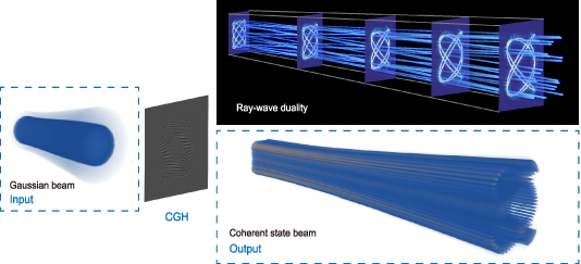
Figure 17. Schematic diagram of digital hologram modulation method for generating SU(2) structured wave-packets. The hologram masks (essentially computer generated hologram, CGH) loaded on spatial light modulator carries the amplitude and phase information of the target light. A Gaussian beam illuminates the CGH. Then the first order of outputting beam contains the target light. After filtering, the intensity distribution of the target light can be collected. The subplot on right top section shows the classical trajectories and transverse intensity distributions at some planes revealing ray-wave duality, the subplot on right bottom section shows the corresponding spatial wave packets.
Download figure:
Standard image High-resolution imageThen, based on the above theory, a specific example is provided to construct an SLM computer generated hologram (CGH) mask for generating a SU(2) geometric mode, that is a trochoidal mode with parameters of P = 1, Q = 4, n = 8, m = 18, and N = 5, as shown in figure 18. Firstly, we prepare a phase blazed grating with a certain period, which is just a wrapped 1D phase slope. The period is selected based actual experimental condition in order to effectively separate the 1st diffraction order (figure 18(a)). Secondly, we superpose the theoretical phase distribution of the on-demand mode onto the blazed grating, and make that into a structured phase grating (figure 18(b)). Thirdly, we multiply the envelope function based on the theoretical amplitude pattern of the on-demand mode (figure 18(c)), then the SLM CGH mask was completed (figure 18(d)). If we illuminate the mask by a nearly-planar wave, e.g. a collimated TEM00 mode at beam waist, and filter the 1st diffraction order, the modulated beam will become the SU(2) geometric mode demanded.

Figure 18. An example to construct an SLM phase mask for generating a SU(2) geometric mode: (a) a phase blazed grating with a certain period; (b) the phase of the SU(2) geometric mode; (c) the amplitude of the SU(2) geometric mode; (d) the SLM CGH mask for generating the SU(2) geometric mode.
Download figure:
Standard image High-resolution imageAs a special structured modes, the SU(2) structured wave-packets are scalar modes. And its light field in any cross section can be represented by:

where A and Φ are amplitude and phase of SU(2) structured wave-packets modes, respectively, and ![$A\subset \left [ 0,1\right ]$](https://content.cld.iop.org/journals/2040-8986/23/12/124004/revision2/joptac3676ieqn317.gif) ,
, ![$\Phi\subset\left[0,2\pi \right ]$](https://content.cld.iop.org/journals/2040-8986/23/12/124004/revision2/joptac3676ieqn318.gif) . The phase function of CGH method [78] is given as:
. The phase function of CGH method [78] is given as:

where  is the inverse function of the first class of first-order Bessel functions, and the maximum value of C for fulfilling
 ![$A = J_{1}[\,f(A)]/C$](https://content.cld.iop.org/journals/2040-8986/23/12/124004/revision2/joptac3676ieqn320.gif) is C = 0.5819.
is C = 0.5819.
where the u0 and v0 are the reciprocal of the period of linear blazed grating in x and y direction, respectively. Now that we have obtained the target SU(2) structured wave-packets in the first diffraction order of modulated light.
In contrast to the SLM, the merit of DMD is the fast speed. The DMD transmission function of the hologram is given as [79]:
where the u0 and v0 have same physical meaning as SLM phase hologram method. The experimental generation of SU(2) geometric modes using DMD was recently reported [82]. And the wave-packets also was isolated and selected in the diffraction order of modulated light. Such digital modulation method can overcome this limitation to generate on-demand the SU(2) structured wave-packets in free space without a cavity [58]. extending advanced ray-wave geometric modes as a powerful and customized toolbox into applications such as optical communication, optical tweezers, high dimensional cryptography, and quantum entanglement.
7. Geometric representations of geometric light
Abstractly geometric representations of complex structured light is convenient for researching their topological evolution and revealing their topological structure intuitively, playing as a salient toolkit to enrich the technologies of optical manipulation and quantum information, particularly pertaining to multi-dimensional geometric light. Thus, a lot of efforts have been devoted to related research.
7.1. Poincaré sphere: from polarization to OAM
Polarization and spatial mode, the two basic DoFs to construct structured light, both have classic graphical representations to describe their evolutions. In particular, the polarization state in two-dimensional qubit space is mapped on the Poincaré sphere:

as shown in figure 19(a). The spatial mode is always given by the OAM state of light, sharing the same qubit formation of the polarization, which can be also mapped on a Poincaré-like sphere [83]:

where  and
and  are the two OAM states with topological charges
  and
and  corresponding to the two poles of Poincaré sphere, see figure 19(b). This representation also plays an important role in quantum optics, because it represent a unit of quantum information (qubit). Therefore the vector beam state is combining the two DoFs together, that is using the tensor product of OAM state and polarization state,
  , thus which can also be represented by a Poincaré sphere, namely higher-order or hybrid-order Poincaré sphere [84, 85]:

as shown in figure 19(c). Therefore, the vector beam, as the two-DoF 2D non-separable state, shares the same formation as the bipartite entangled state in quantum mechanics. The conventional structured light are limited by two DoFs, spatial mode (OAM) and polarization. While we can find a way to generalize the description of structured light with extended DoFs and higher dimensions. In the OAM Poincaré sphere model, we actually only consider the azimuthal mode of a laser beam, but a complete description of laser beam should includes three modes: one longitudinal mode  and two transverse modes (azimuthal
  and radial
  modes, or horizontal
  and vertical
  modes). The longitudinal mode determines how the beam is divergent upon propagation. The two transverse modes determine the singularity distributions along the two transverse directions. A generalized model considering the three modes can be exploited by the SU(2) transformation [86–88],
where  ,
,  ,
,  ,
,  is the Wigner d function, and
  is LG mode with radial and azimuthal indices of ρ and
  . The generalized eigenstate of equation (96) forms a family of HLG modes, and which can also be mapped on a modal Poincaré sphere with full OAM evolution, as shown in figure 20(a), the subplots on north and south poles are LG modes with opposite OAM. The subplots on equator are HG modes and others are HLG modes. The longitudinal mode l cannot revealed by the transverse pattern but impacts on how the beam is divergent along the longitudinal direction, as shown in figures 20(b)–(d), which plays an important role in superposing complex longitudinally variant structured beams (see section 7.3 for more details). This modal Poincaré sphere representation is the most general description of scalar freespace eigenmodes under the general SU(2) symmetry of paraxial beam system. While, it is also a valuable direction to further generalize the modal, coupled with the polarization Poincaré sphere, to include more kinds of intriguing vectorial structured light beams.
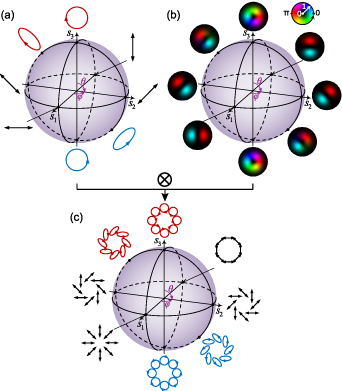
Figure 19. (a) Poincaré sphere represents the polarization state of light. (b) Poincaré sphere represents the OAM mode of light, The Hue color refers to phase from 0 to 2π and the darkness/brightness refers to the intensity from 0 to 1. (c) High-order Poincaré sphere represents complex the vector field of light.
Download figure:
Standard image High-resolution image
Figure 20. (a) Modal Poincaré sphere represents the HLG eigenmode with OAM evolution with example of indices  . (b)–(d) the longitudinally divergent profiles of LG, HLG, and HG modes.
Download figure:
Standard image High-resolution image7.2. Ray-optics Poincaré sphere for structured Gaussian eigenmodes
Paraxial ray families crossing the focal plane can be represented as dual-parameter families of ellipses, parametrized by curves on an ray-optics Poincaré sphere for rays with diverse caustic structures. With deeper understanding of structured eigenmodes, any HLG mode can be described in terms of the ray family in which each ray is specified by the values of two periodic parameters so as to be mapped on such Poincaré sphere, which has been proposed in the context of semiclassical estimates for structured light [89–92]. For example, the behavior of a propagating HG mode as figure 21(a) can be analogue to a corresponding ray caustics as figure 21(b).
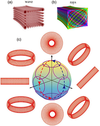
Figure 21. (a) The spatial wave packet of a propagating HG mode and (b) corresponding analogue caustic representation including a set of rays. (c) The ray-optics Poincaré sphere with corresponding rays modes shown at selective points, and corresponding Poincaré paths for various points are marked as purple circles. (a), (b) Reprinted (figure) with permission from [92], Copyright (2018) by the American Physical Society.
Download figure:
Standard image High-resolution imageIn ray-optics Poincaré sphere, a ray caustic mode is not represented by a single point on the sphere, but by the point together with a closed loop surrounded to it over the sphere model, namely Poincaré path, as shown in figure 21(c). In paraxial ray optics, each ray can be expressed as  , where
  is the transverse coordinate and
  is the transverse direction vector. At z = 0 plane,
  ,
,  (
( , where v is an unit vector defined on Poincaré sphere as
  , where
  determines the points on Poincaré sphere,
  ,
,  . For fixed
  ,
,  is a fixed point on Poincaré sphere, Q traces out an ellipse. For varying
  , if
, if  can form a closed Poincaré path, the trajectories of Q consists of a series of ellipses corresponding to generalized HLG beams, then the wave fields can be estimated only based on ray description validly [51, 89, 93].
In addition to the conditions for HLG beams, a generalized model of the ray-optics Poincaré sphere for more general structured Gaussian beam was proposed recently [94]. The general structured Gaussian beam with total order N can be expressed as  , where
  represents LG mode with total order number N and angular order
  , expansion coefficients
  are used to define Nth-order Majorana polynomial as
  , where the zeros of Majorana polynomial map onto so-called modal Majorana sphere through a stereographic projection
  . Thus any structured Gaussian beam could beniquely represented by N points on modal Majorana sphere. This representation method reveals hidden symmetries of structured Gaussian beams and provides a deep physical insight for geometric phases. Note that the Majorana sphere and Poincaré sphere have fundamental difference to represent a mode. The Poincare sphere represent a mode by a point on it, but the Majorana represent a mode by a special set of points on it. That is a manifestation that majorana model can open higher dimensions of structured beams [94, 95].
7.3. General SU(2) Poincaré sphere for ray-wave structured light
In above two sections, elegant models are reviewed to map arbitrary-order SU(2) eigenmodes, i.e. HLG modes, onto a Poincaré sphere and reveal the general OAM evolution, especially in both wave and ray treatment. Although each eigenmode has corresponding ray caustic representation, the caustics is just a phenomenological interpretation of the wave mode propagation. In contrast to this, the SU(2) coherent state mode with ray-wave duality, as well-defined superposed state of a set of eigenmodes, can show more rigorous ray-wave coupling representation, where the wave pattern is exactly coupled with the distribution of rays. Hereinafter, the modal of general SU(2) Poincaré sphere will be shown to represent the coherent state ray-wave structured light.
Since arbitrary-order HLG eigenmodes can be mapped on Poincaré sphere, the SU(2) coherent state, as the superposed wave-packet with a special set of eigenmodes can also be mapped on Poincaré sphere, to further generalize the Poincaré sphere model, namely, SU(2) Poincaré sphere [96]. Based on equation (96) and, the closed-form expression can be given by:
which enables us to map the SU(2) coherent state onto a new generalized Poincaré sphere, namely, a SU(2) Poincaré sphere, as shown in figure 22 for a example case of multi-path geometric mode with  , which vividly illustrates the OAM evolutions of both the spatial geometric wave packet together and the coupled 6-ray caustics. Also the SU(2) Poincaré sphere has its higher-order generalization to represent multi-HLG and Lissajous-to-trochoidal geometric modes, the diverse generalized forms of eigenmode Poincaré sphere and SU(2) Poincaré sphere are shown in figures 23(a) and (b), respectively. Note that a diagram showing how the various kinds of SU(2) beams relate to each other can refer to figure 11. As a more generalized form of eigenmode Poincaré sphere, SU(2) Poincaré sphere opens new dimensions to reveal the topological evolution of complex ray-wave structured light, paving the way to the new studies of spin-to-orbital conversion, complex mode entanglement, optical encoding and communication, and geometric phase transition.
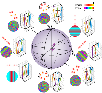
Figure 22. SU(2) Poincaré sphere represents the ray-wave geometric mode, for both evolutions of spatial wave pattern and ray trajectory.
Download figure:
Standard image High-resolution image
Figure 23. (a) Eigenmode Poincaré sphere representations for polarization states, OAM mode states and HLG modes in inner, middle, and outer inserts, respectively. The poles represent right- and left-handed circular polarizations, right- and left-handed-OAM LG modes and higher-order LG modes of opposite OAM. The equator linear polarization, HG modes and higher-order HG modes. (b) SU(2) Poincaré sphere representations for multi-path, multi-HLG, and Lissajous-trochoidal ray-wave geometric modes.
Download figure:
Standard image High-resolution image8. Other kinds of SU(2) structured light
The SU(2) symmetry in structured light is so general that there are many other extensions not covered above. In addition to the freespace geometric beams at frequency degenerate states, there are still many other kinds of exotic SU(2) structured light with general conditions. For instance, when a basic multi-spot ray-wave SU(2) geometric mode is tuned from a pure frequency-degenerate state into a quasi-degenerate state, multiple spots in the pattern can be connected to each others to form a polygonal vortex beam. We can introduce astigmatic effects onto an basic SU(2) geometric mode to generate astigmatic SU(2) geometric mode with more general longitudinally variant patterns. We can also can replace trivial freespace HLG eigenmodes state into nontrivial nondiffracting modes and waveguide modes and so on to explore more intriguing forms of SU(2) structured light. Hereinafter, these exotic SU(2) structured light will be introduced in more details.
8.1. Polygonal vortex beams
The frequency-degenerate theory is established under the assumption of monochromatic light field, while the actual laser beams are always quasi-monochromatic with a spectral linewidth. Thus, a mode in degenerate state cannot drastically collapse to a non-degenerate state when the frequency-degenerate state is adjusted to a condition in the vicinity of degenerate state. It was reported that, at a quasi-degenerate state, the original multiple spots of the transverse pattern of SU(2) vortex can be connected to each others to form an exotic polygonal shape, i.e. the polygonal vortex beams [67], see figure 24. The quasi-frequency-degenerate (QFD) wave-function to describe the mode behavior in the vicinity of frequency-degenerate state [67]:
which can be seen as a superposition of a pure SU(2) degenerate HLG modes and some additional HLG modes, where the coefficient qK
represent the weights of the superposed  modes. The physical meaning of parameter qK
can be interpreted as the component of the decomposed HG mode
modes. The physical meaning of parameter qK
can be interpreted as the component of the decomposed HG mode  outside of the pure SU(2) wave-packet, see simulation examples in figures 25(a1)–(a4).
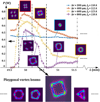
Figure 24. At a quasi-degenerate state, the original multiple spots of the transverse pattern of SU(2) vortex can be connected to each others to form an exotic polygonal shape, i.e. the polygonal vortex beams.
Download figure:
Standard image High-resolution image
Figure 25. Exotic SU(2) structured light. (a) Quasi-degenerate state SU(2) geometric beam, the transverse distributions for (a1), (a2) ( ) and (a3), (a4) (
 ). (b) Astigmatic hybrid SU(2) geometric beam, the transverse distributions (
 ) at z = 0 plane for (b1), (b2) and at far field for (b3), (b4). (c) Resonate SU(2) geometric beam, the transverse distributions for (c1), (c2)
  and (c3), (c4)
  . (d) Localized SU(2) geometric microlaser mode, the transverse distributions for (d1)(d2) φ = 0 and (d3)(d4)
  . (e) Eigenmodes of SU(2) coupled commensurate harmonic oscillators,
  for (e1), (e2) and
  for (e3), (e4). Rows 1,3 for intensity distributions and rows 2,4 for phase distributions, respectively (colormap: darkness to brightness means 0 to 1 for intensity,
  to π for phase, 0 to
  for P1 and
  to π for P2, respectively).
Download figure:
Standard image High-resolution imageIn a optical resonator, the condition of a pure SU(2) wave-packet in degenerate states is more rigorous than that of a HG mode in non-degenerate states. Therefore, it is rational to understand the quasi-degenerate states as that some extrinsic HG modes outside a pure SU(2) wave-packet are mixed in. The polygonal vortex beams can be demonstrated with the intrinsic LG bases, which can be realized by a an external  -cylindrical-lens astigmatic mode converter. Additionally, we note that the occurrence of degenerate states is not only determined by the fraction, but also impacted by factors such as pump power, pump beam size, off-axis displacement, gain medium, etc [97]. For the same fraction, the laser can possibly perform as a degenerate state or a quasi-degenerate state or even a non-degenerate state for different gain media, pump power, off-axis displacement, etc which is related by the form of quasi-degenerate parameters qK
. However, such model cannot predict the value of qK
for the given polygonal geometry. Recently, some improved models were proposed that can make the polygonal vortex beams exactly more strictly coupled with the given polygonal geometry [97, 98]. However, which cannot be related to the corresponding frequency-degenerate state. Thus the complete theory for polygonal vortex beams is still to be explored.
-cylindrical-lens astigmatic mode converter. Additionally, we note that the occurrence of degenerate states is not only determined by the fraction, but also impacted by factors such as pump power, pump beam size, off-axis displacement, gain medium, etc [97]. For the same fraction, the laser can possibly perform as a degenerate state or a quasi-degenerate state or even a non-degenerate state for different gain media, pump power, off-axis displacement, etc which is related by the form of quasi-degenerate parameters qK
. However, such model cannot predict the value of qK
for the given polygonal geometry. Recently, some improved models were proposed that can make the polygonal vortex beams exactly more strictly coupled with the given polygonal geometry [97, 98]. However, which cannot be related to the corresponding frequency-degenerate state. Thus the complete theory for polygonal vortex beams is still to be explored.
8.2. Astigmatic hybrid SU(2) geometric beams
Recently, an exotic kind of structured light, astigmatic hybrid SU(2) geometric beam, has been proposed in the perspective of classical trajectories [99], providing a physical insight in the picture of semi-classical ray-wave duality [100, 101]. The hybrid planar geometric beam would evolve to circular vortex geometric beam during propagation after passing through the cylindrical lens, as shown in figures 25(b1)–(b4). Selecting z = 0 as the position of the cylindrical lens and  , the mathematical formulas of astigmatic hybrid classical trajectories cluster
  has been derived for characterizing the topological evolution of astigmatic hybrid SU(2) geometric beam as [99]:

where N is the transverse indices,  ,
,  is the cluster of classical trajectories of astigmatic geometric beam, which can be mathematically expressed as [99]:
where  ,
,  ,
,  are astigmatic Gouy phases in x'- and y'-axis,
  ,
,  are astigmatic Gaussian beam waist parameters [102, 103]. Then we can get the spatial wave-packet of astigmatic geometric beam by substituting equation (100) into equation (53) as
  (
( ). And the spatial wave-packet of astigmatic hybrid geometric beam can be expressed as
  . Particularly, an exotic vector structured light, vector astigmatic hybrid SU(2) geometric beam can be constructed by modulating the polarization of
  and
and  , which can realize longitudinally-variant spatial twisted ray-wave structure and vector singularities upon propagation, as shown in figures 25(b1)–(b4), where
  ,
,  and
and  are left-handed circular polarization and vertical polarization. In order to reveal more vector properties about vector structured light, two parameter has been defined as
  and
and  [62]. The spatial wave-packet located on each astigmatic ray can be obtained by substituting equation (100) into equation (52). Figures 25(b1)–(b4) show the exotic longitudinally-variant property of vector astigmatic hybrid SU(2) geometric beam, evolving from planar geometric beam without singularities at z = 0 plane to vortex geometric beam with multi-singularities at far field, which is significant for further exploring the related applications in longitudinally variant polarized optics, optical manipulation and communication, etc [8, 104–106]. Besides, the exotic vector astigmatic hybrid SU(2) geometric beam can have more controllable DoFs by modulating the polarization of sub-beams [99].
8.3. Resonate SU(2) geometric beams
SU(2) geometric beams are essentially coherent superposition of a series of eigenmodes with sub-Poisson distribution weights and same frequency. Therefore, the transformations of SU(2) geometric modes can be realized by converting eigenmodes. For example, the planar geometric modes can be converted to circular geometric modes by converting HG modes to LG modes. Furthermore, LG modes can be converted into Bessel modes by using an axicon [107] leading to an exotic kind of geometric modes, i.e. resonate geometric modes [108], as shown in figures 25(c1)–(c4). In fact, Bessel beams are propagation-invariant solutions in cylindrical waveguide [109]. Because the confinement of waveguide can be regarded as a circular billiard for light, the resonate geometric modes, coherent superposition of nearly degenerate Bessel beams, can be regarded as coherent state related with a circular quantum billiard [110], which can be expressed as [108, 110]:
where  is angular normalization factor,
  is radial normalization factor derived from
 ![$N_{n,m}^2~\int_0^R [{J}_{n}(k_{n,m}r)]^2 r{d}r = 1$](https://content.cld.iop.org/journals/2040-8986/23/12/124004/revision2/joptac3676ieqn394.gif) ,
,  is the first kind of Bessel function with indices n,
  ,
,  ,
,  , and
, and  is mth zero of
  [111].
8.4. Localized SU(2) geometric microlaser beams
SU(2) coherent state can not only be constructed in free space, but also existed in localized waveguide or microcavities. In construct to the eigenmodes in freespace, the eigenmodes in a localized waveguide require boundary conditions determined by its geometric shape. The frequency-degenerate set of eigenmodes in a waveguide is also existed and can play as the eigenstates for constructing the SU(2) coherent state wavepacket. For example of a 2D square waveguide with side length of a, rather than the HG mode solutions in freespace, the eigenmode can be solved as [112]:
where  , which can also act as eigenstates to construct an SU(2) coherent state [113, 114]:
Such micro-scale localized SU(2) geometric beam also harness intriguing ray-wave duality, that the corresponding classical trajectory includes the rays bouncing back and forth in a waveguide with prescribed geometric orbits [115]. Figures 25(d1)–(d4) show some patterns of micro-scale localized SU(2) geometric beams (N = 2,  , M = 0). The earliest localized SU(2) geometric mode was realized in a electric pumped square waveguide as a vertical cavity surface emitting laser (VCSEL), where the lasing pattern is described as quantum billiards [114, 116]. The quantum billiard effect was also realized by triangle waveguide, forming more general patterns and intriguing vortex lattices effect [113]. With the development of microlaser, the localized SU(2) geometric mode manipulated in a VCSEL can emit the SU(2) structured light from waveguide into free space [117, 118].
Recently, the SU(2) structured light realized in microlasers has hatched tremendous attentions in fundamental physics. The ray-wave light structure in microcavities provided an effective way to realize high-power directional emission from the microscale [119]. Also, combining the advanced organic single-crystalline materials, the crystalline microresonators enables more intriguing whispering-gallery modes with improved tunable polygonal geometries [120]. It was also unveiled that the ray-wave duality in microcavities provide new opportunities to study fundamental physical effects of wave chaos [121] and non-Hermitian physics [122], which was also recently applied to suppressing spatiotemporal instabilities of microlaser [123]. The ray-wave structured light in semiconductor laser was also used as a powerful tool to control complex coherent modes [124, 125] and directional emission [126], enabling new applications in imaging and wavefront shaping [127].
8.5. Commensurate harmonic oscillator coupled geometric beams and beyond
These kinds of exotic SU(2) structured light mentioned above are the cases of classical structured light corresponding to SU(2) coherent state. Here we will introduce another exotic structured light with SU(2) symmetry, an eigenstate of SU(2) coupled commensurate harmonic oscillator [128]. For a generalized anisotropic Hamiltonian in equation (26), the coupling term  can be regarded as SU(2) coupling interaction and the corresponding eigenstate can be expressed as [128]:
where  represents eigenstate of isotropic
  corresponding to HG modes with indices
  ,
,  is wigner d coefficient,
  ,
,  ,
,  . Eigenmodes corresponding to anisotropic Hamiltonian
  are a linear superposition of HG modes, where the intensity are located on Lissajous curves from single to multiple trajectories with n1 increasing, as shown in figures 25(e1)–(e4). The simulation parameters are as N = 30,
  ,
,  ,
,  .
.
Based on the above discussions, the SU(2) mathematical model with multiple controllable parameters can derive diverse exotic geometric modes with infinite possibilities. Besides the above four typical forms, many new modes were emerged very recently, polygonal Airy beams [129], frequency-degenerate bottle beams [130], Siegman's elegant laser modes [131], standing-wave and traveling-wave unified geometric mode [82], to name a few. There are definitely many hidden parameters in SU(2) symmetry to be opened to explore more intriguing geometric modes in the future.
8.6. Classically entangled SU(2) structured light
What is classical entanglement? Entanglement, a purely quantum mechanical phenomenon, was originally coined to describe quantum correlations that can be shared between spatially separated multi-particle systems. A defining characteristic of such systems is nonseparability: mathematically, the wavefunctions of entangled systems cannot be written as separable products of the individual subsystems. An typical example is a Bell states,
where the states  and
and  form an information basis for the subsystem A and B. A consequence of equation (106) is that the two systems cannot be written as separable product, hence it is nonseparable. In classical regime, nonlocal interaction at a distance is not existed, but nonseparability as an mathematic relation can be widely applied. The classical entanglement describes systems where the nonseparability or equivalently entanglement, occurs between the internal DoFs of particles. In optics such similarities have been discussed at length in [132–135]. Typical examples of a classical entangled light are vector vortex beams, where the correlations between the polarization and spatial components mimick two-particle maximally entangled Bell states:
Here the labels A and B mark the spatial and polarization components just as one would a composite system of two particles. Here the difference is that the kets mark the DoFs of each single photon in the field and not spatially separated photons. Also notice that the field are completely separable for  .
.
Conventionally, a vector vortex beam fulfill the form of bipartite classical entanglement, as the Bell state, with two DoFs of spatial mode and polarization, see figure 26 left. Now, SU(2) structured light opens an new platform to construct more intriguing classically entangled states, because it harnesses more intrinsic DoFs due to its unique ray-wave geometric structure. For instance, a ray-wave SU(2) geometric beam can have ray oscillating directions and locations to be the extended DoFs. A multi-axis vortex SU(2) geometric mode can have not only central OAM but also partial OAM along sub-rays as extended DoFs. Hereinafter we demonstrate how to use the intrinsic DoFs of SU(2) structured light to represent multi-partite classically entangled state, see figure 26 right, beyond the bipartite Bell state.

Figure 26. A conventional vector vortex beam as the form of bipartite Bell entangled state and the novel SU(2) vector beams as the form of multipartite Greenberger–Horne–Zeilinger (GHZ) state.
Download figure:
Standard image High-resolution imageFor example at  (
( ) we used in the main text, positive and negative W-shaped trajectories coincide exactly, i.e. the positive and negative oscillating states are expressed by:

as shown in figure 2 in the main text. Additionally, in the four periodic round-trips, two share the first bouncing location and other two share the second one, i.e. the round-trip location states are expressed by:

The output states of various rays can be expressed by the corresponding positively longitudinal propagation components of product states between the direction and location states, which are given by:
The ray trajectories in a complete oscillation and the output ray states from cavity are shown in figure 27. In our setup, the concave mirror is the laser output mirror, thus only the forward-propagation states are observable, as the four output ray states marked in figure 27.
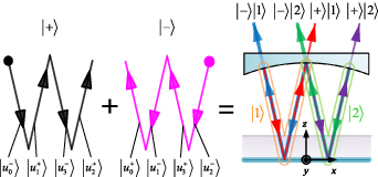
Figure 27. Trajectory direction and location states. The ray orbit components for the positive and negative x-direction construct the trajectory for the direction states  and
and  , and the two
  and
and  construct a complete oscillation in a degenerate laser cavity. The output ray states can be represented by the product states of direction and location states.
Download figure:
Standard image High-resolution imageThe SU(2) geometric vector beam can be expressed in the high-dimensional Hilbert space using the new DoFs from ray-wave representation. For instance of the geometric mode in degenerate state  , the geometric vector beam can be represented by trajectory states:
where the state of polarization  is two dimensions, which can be linearly expanded by bases of
  and
and  . Therefore, the SU(2) vector beam of equation (111) is expressed in 8-dimensional space with bases of
  ,
,  ,
,  ,
,  ,
,  ,
,  ,
,  , and
, and  .
.
We can control the SU(2) geometric beam into ray-like state and then make special modulations to realize various classical Greenberger–Horne–Zeilinger (GHZ) states, the maximally entangled states for multiple particles, see equations (112)–(115), as specific cases:
-
: , , , and ;
-
: , , , and ;
-
: , , , and ;
-
: , , , and ;
-
: , , , and ;
-
: , , , and ;
-
: , , , and ;
-
: , , , and ;


where the GHZ states are given by:
The 3D intensity patterns of various GHZ states with various polarization projection states ( ,
,  , π, and
  ) are shown in figure 28, where we set
  in simulation. When the vortex geometric mode is reduced into planar geometric mode, i.e. Nx
or
in simulation. When the vortex geometric mode is reduced into planar geometric mode, i.e. Nx
or  , we can directly use intensity pattern
  to observe the interference effect among sub-orbits, as shown in figure 5 in the main article for various GHZ states. By experimentally measuring the amplitude, phase, and polarization of each orbit (the phase can be reconstructed by the interference pattern among various basic states), we can evaluate the experimental state:
reconstitute the density matrix  for each experimental GHZ state, and calculate the fidelities
  and
and  (
( ) comparing with the theoretical density matrices of GHZ states.
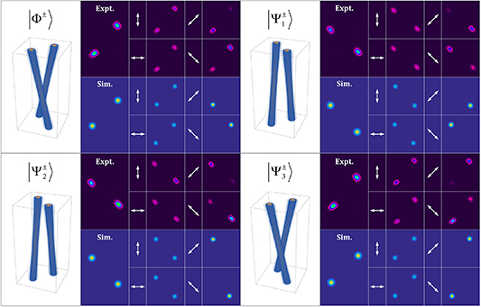
Figure 28. Control of four maximumly entangled groups in GHZ states. The experimental and theoretical results of four general SU(2) vector beams corresponding to the four maximumly entangled groups in classical GHZ states. The white arrow means the allowed polarization orientation of the polarizer. The plot on the left for each group shows the theoretical spatial wave-packet of the corresponding SU(2)-like vector beams.  : the SU(2)-like vector beam with diagonal intensity pattern where
  orbit with diagonal polarization
  orbit with anti-diagonal polarization;
  : anti-diagonal intensity pattern,
  orbit with diagonal polarization
  orbit with anti-diagonal polarization;
  : anti-diagonal intensity pattern,
  orbit with diagonal polarization
  orbit with anti-diagonal polarization;
  : diagonal intensity pattern,
  orbit with diagonal polarization
  orbit with anti-diagonal polarization.
Download figure:
Standard image High-resolution imageHereto, we can already generate a complete set of GHZ states from a laser, sharing the same form of three-photon quantum entanglement. The general SU(2) geometric modes also have potential to be used to generate even higher-dimensional entanglement states with the form of N-photon (N > 3) quantum entanglement. To this end, we should find more DoFs to extend the dimension in classical entanglement such as OAM. As shown in figures 29(a)–(d), two SU(2) geometric modes with opposite OAM can be superposed together fulfilling a complete oscillating trajectory in a cavity, which can also be experimentally realized [72]. After inhomogeneous intensity and polarization modulation, this kind of general SU(2) geometric modes should be represented in 16-D Hilbert space like the 4-photon quantum entanglement:
with 16 (4 partite and 8 maximumly entangled group) GHZ states as eigenstates (just show the first maximumly entangled group here):

Figure 29. Towards higher-dimensional classical entanglement. Spatial SU(2) geometric beams can carry OAM and the OAM can be a DoF manifesting additional dimensions in classical entanglement. (a) A superposed trajectory on SU(2) state  including the positive-OAM and negative-OAM decomposed SU(2) trajectories, (b) which can exactly fulfill a complete SU(2) oscillation in a degenerate cavity. (c) Based on the ray-wave duality, the corresponding geometric mode can be represented by the superposition of a positive-OAM and a negative-OAM vortex SU(2) beams (the topological phase manifesting the OAM and intensity wave-packet are shown in the inserts). This generalized beam can be expressed into 16-dimensional state with 4 DoFs and 16 eigenstates noted in (d). (e) An exotic multi-vortex SU(2)-structured mode is obtained by the superposition of two multi-vortex SU(2) geometric modes with opposite main-OAMs, and the sub-OAM carried by each sub-ray mode can also play as a new DoF, where the notation
  refers to the OAM topological charge at the beam center (as marked by the yellow dashed circle) and
  the OAM topological along each sub-ray (as marked by the purple dashed circle). This generalized beam can be expressed into 32-dimensional state with 5 DoFs and 32 eigenstates noted in (f).
Download figure:
Standard image High-resolution imageFor exploring more DoFs to extend the dimension in classical entanglement, we can utilize multi-LG SU(2) beams [48, 49], where LG beams replace the Gaussian beams along SU(2) orbits in a geometric mode based on ray-wave duality. Thus, there is a main OAM state  along the propagation axis, but also OAM
  along an SU(2) orbit. The sub-OAM
  has potential to be a DoF to reach higher-dimensional entanglement. As shown in figures 29(e) and (f), exotic beams can be obtained by the superposition of two multi-LG SU(2) beams with opposite main OAM, realizing the 32D entangled stated with 5-partite 16-group GHZ states as eigenstates (just show the first maximumly entangled group here):
Besides finding more DoFs, increasing the number of orbits can also extend the dimension. The above demonstrations are all at degenerate state  . If we can control higher-order degenerate state
  (P and Q are co-prime integers, Q is even), the general SU(2) geometric modes would be extended into 4 Q-dimensional space:
Involving the sub-OAM in multi-LG SU(2) beams, that can be further extended into 8 Q-dimensional space:
The realization of high-dimensional classical entanglement can pave the way for developing a myriad of novel applications of quantum mechanism using classical light.
9. Potential applications
In recent years, the creation and control of various SU(2) structured light has made major breakthrough with more DoFs of light tamed, which has promised the advances in a myriad of applications. However, the development of these potential applications is in its infancy. Thus, it is important to outlook on some applications in this section.
9.1. Laser machining and fabrication
The recent development of solid-state laser allows not only the generation of various SU(2) structured light but also higher output power and energy beyond the threshold to be applied in laser machining and fabrication [140]. Many advanced laser technologies, e.g. Q-switching and mode-locking, were used to generate high-power and large-energy pulse from a laser, and these methods were applied in structured light laser to generate high-power and large-energy SU(2) structured light. The self-mode-locking effect of Nd:YVO4 crystal was applied in solid-state laser to generate the SU(2) structured ultrashort pulse with pulse-width about 30 ps and the average output power at 500 mW, which is applied for both planar geometric modes [141] and vortex geometric modes [142]. Then, the passively Q-switching scheme was used to further improve the output power with output energy and peak power towards over 100 μJ and 10 kW [143]. Recently, a method for optimizing high-power geometric mode is proposed, considering the thermal lensing effect in the gain medium, which allows the output of geometric mode to hold several-Watt-level average power [144]. Soon after, this power-optimizing method was applied in higher-order SU(2) structured light laser, which realized the Watt-level output and complex SU(2) structure simultaneously [49]. Such high-power output optimization was also verified in higher-order Lissajous structured modes [145]. In short, the recent advance of high-power SU(2) structured light laser has promised the enough power output to be applied in laser machining and fabrication. The light with complex spatial structure, especially the OAM structure, has a great potential to be used in advanced chiral material processing and fabrication [146]. While the SU(2) structured light has more versatile spatial chiral structure than the common OAM beam to extend the frontier of material fabrication, which leads to advanced photonic devices such as metamaterials, ultra-sensitive detector, and chiral chemical composites. For example, the polygonal vortex beams can be used to produce complex 3D spiral polygonal microtubes for realizing novel polymerized functional devices [136], see figure 30(a).

Figure 30. Examples of potential applications. (a) Laser machining and fabrication: two-photon polymerization with femtosecond vortex beam for direct laser writing of microtubes. Reprinted from [136], with the permission of AIP Publishing; (b) complex tweezers and multi-particle manipulation: the trapping potential and force distributions induced by pulsed SU(2) cylindrical vector beams. Reprinted with permission from [137]. Copyright © 2018, American Chemical Society; (c) topological photonics: SU(2) twisted wave packets of the right- and left-traveling modes in a Weyl semimetal. Reproduced from [138]. CC BY 4.0; (d) high dimensional encoding and high-capacity communication: simulating multiplexed vortices passing through a Dammann vortex grating. Reproduced from [139]. CC BY 4.0.
Download figure:
Standard image High-resolution image9.2. Complex tweezers and multi-particle manipulation
With the application of optical force in biology, physics and chemistry, numerous optical tweezers and optical trapping with different properties appeared in people's field of vision [147]. Optical tweezers commonly refer to utilizing gradient and scattering forces of electromagnetic fields to manipulate micro- and nano-particles [148]. The customization of pattern and OAM has become the focus of research [149–151], including multi-spots optical trapping [149, 152], polygonal optical trapping [153], three dimensional optical trapping [154, 155], etc. Utilizing structured light to manipulate various micro- or nano-particles has been a hot topic in past few decades, such as Mathieu beams [156] and Ince–Gaussian beams [157] for 3D assembly of micro-particles, perfect vortex beam and asymmetrical vortex Bessel-Gaussian beams [158] for trapping micro-particles [159], non-diffracting Airy beams array for optical trapping [160] and many other advanced optical manipulations based on complex beams [152, 153, 161, 162]. SU(2) geometric beams with complex and customized spatial structure, including the OAM structure and intensity shape, have a great potential to be a toolkit in advanced optical manipulation. Based on holographic method, the generation and dynamic control of SU(2) geometric beams can be accurately and rapidly realized with high-quality via SLM [58], which is significant for flexible and controllable optical trapping and manipulation [163]. Besides, polarization and nonlinearity of light beams can also be practical tools to realize optical trapping and manipulation [137], see figure 30(b). The complex polarization structures of SU(2) geometric beams with multiple DoFs have been constructed [62, 164], demonstrating the potential applications of SU(2) geometric beams with exotic hybrid vector structure in complex tweezers and multi-particle manipulation. Researching the nonlinearity of SU(2) geometric beams would be an attractive topic to reveal more significant applications in optical manipulation.
9.3. Topological photonics
Since the discovery of topological phases and topological insulators in modern natural science, topological phenomena are ubiquitous in physics, with explorations spanning areas from condensed-matter physics to physical cosmology [165, 166]. In which, an important branch is topological photonics, that emulates concepts in condensed matters and topological insulators into optical or photonic systems [167–170]. The frequency-degenerate cavity and the enabled SU(2) geometric modes also play import role in extending the frontier of topological photonics. It was proposed that the photonic Landau levels can be realized in an SU(2) geometric mode laser cavity, see figure 31(a), with controlled frequency-degenerate states, see figure 31(b), exactly emulating the fermion energy level motion in a synthetic magnetic field [171]. Due to the similar topology of topological Chern insulators, see figures 31(c) and (d), the Landau levels of SU(2) structured light laser can be used to realize electromagnetic and gravitational responses of photonic quantum Hall materials, enabling enable precise characterization and metrology of topological matter in photon fluids [172]. Moreover, with light-mater interaction using such topological effect of structured light, the photonic Laughlin mater can be made to reveal deeper ordered states and new DoFs in light [173, 174].
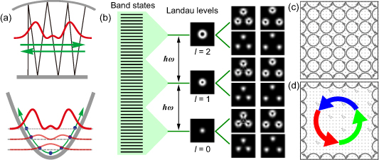
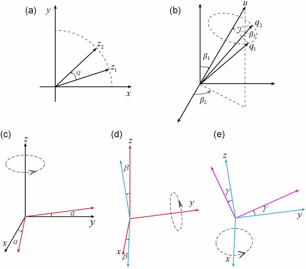
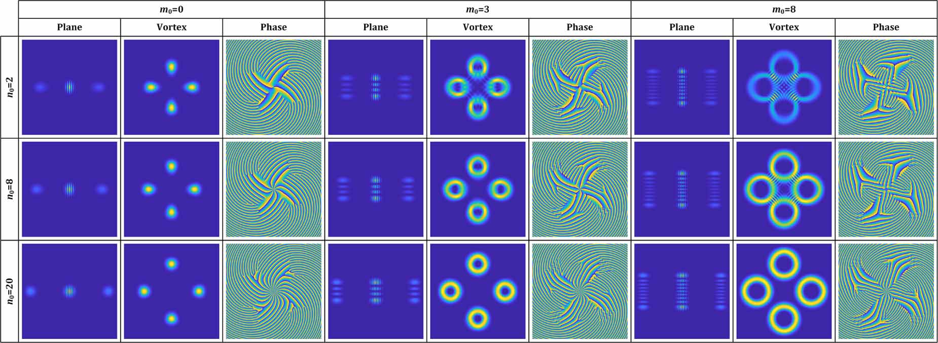
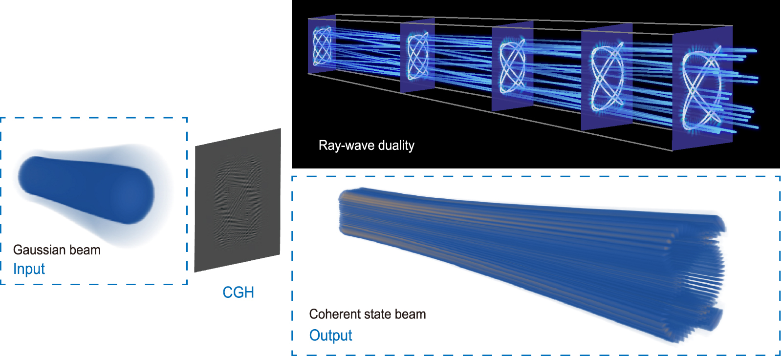
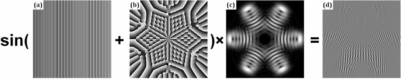
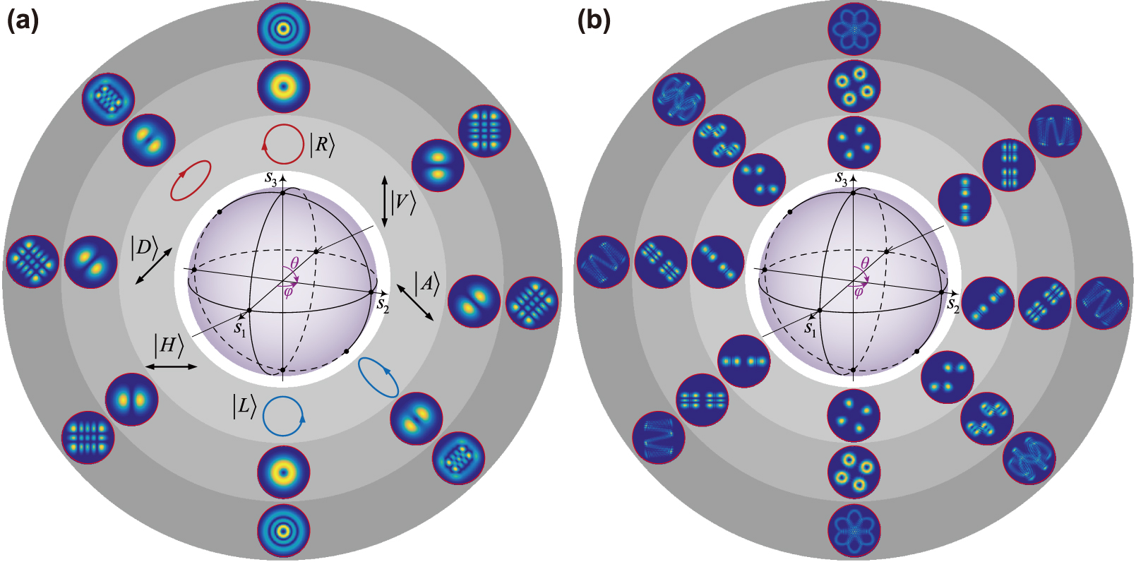
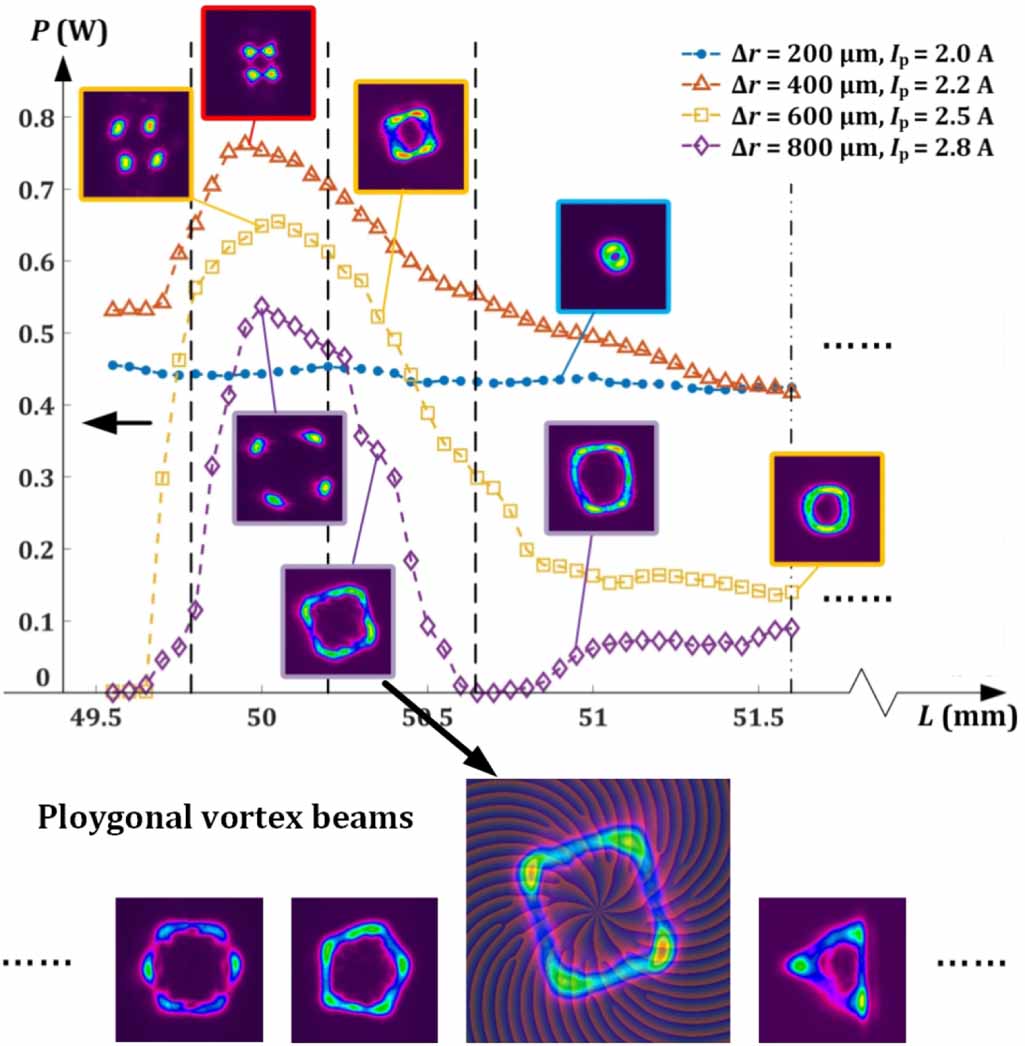
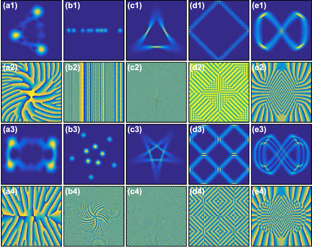
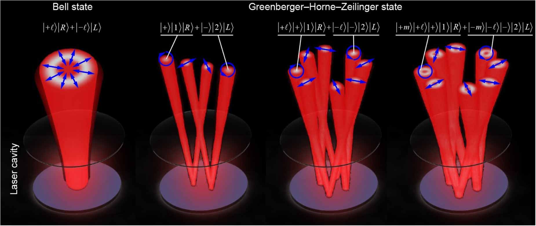
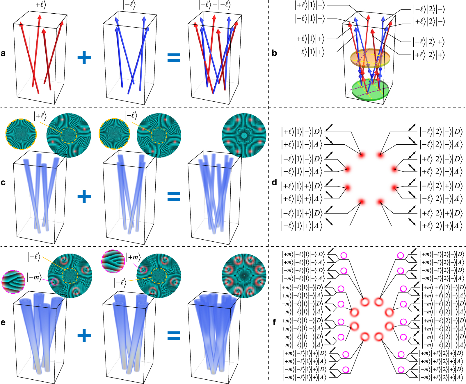
Figure 31. (a) A customized ray-wave frequency degenerate state in laser resonator, which can realized by a manifold rotating-mirror geometric solid-state cavity, (b) the structured laser emission of various frequency-degenerate SU(2) geometric modes fulfills a mechanism of photonic Landau levels [171]. (c) The topological structure in real space of photonic Landau level laser shares a similar form of k-space structure of a topological Chern insulator, (d) and the direct measurement of the Chern number in bulk topology requires a disorder-insensitive probe of bulk chiral nonreciprocity [172].
Download figure:
Standard image High-resolution image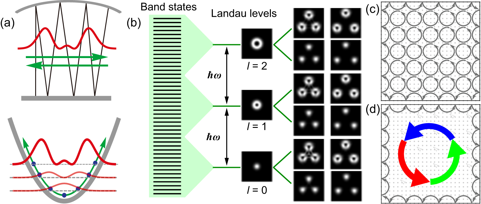
Besides, significant advances have been made in high dimensional topological photonics [175, 176]. A concept of three-dimensional (3D) topological twistronics has been proposed based on a 3D layered systems with a constant twist angle between successive layers, providing a novel method to realize topological physics [138], see figure 30(c). SU(2) geometric beams also have 3D spatial distortion property in free-space propagation, which could be used to simulate the 3D topological twistronics to research high-dimensional topological physics. Active topological photonics is also a rapidly developing field due to its wide applications in topological lasers, topological edge modes, non-Hermitian topological physics, and singular optics, etc [177, 178]. SU(2) geometric beams can provide richly exotic topological phase structure for active topological photonics. Although most of advances in topological photonics is oriented to theoretical research, some technical works have been made. For example, terahertz topological photonics was used to realize low-cost, efficient and high-speed on-chip communication [179].
Topological photonics is a very attractive topic for many frontier fields such as topological quantum photonics [180], non-Hermitian topological photonics [181], topological insulator laser [182, 183], toroidal light [184, 185], optical skyrmions and bimerons [186, 187], and calling for more fundamental ideas and exciting applications [188]. Exploring the classical structured light to simulate the topological photonics would be a significant direction and SU(2) geometric beams could offer a powerful tool to research classical simulation of topological photonics.
9.4. High-capacity encoding and communication
High dimensional encoding and high-capacity communication are attractive topics and structured light applied in related fields has been researched for few decades [20, 105, 189, 190]. Various properties of structured light such as OAM evolution and spatial mode structure have been demonstrated that can be used to improve high-dimensional cryptography and secure communication [191–193]. The spatial topological structure is significant for mode-division multiplexed method because spatial mode have shocking infinite DoFs in theory [194–196]. SU(2) geometric beams have rich spatial mode structures which can be accurately controlled by a series of parameters, which is a great advantage for expanding encoding dimensional and communication capacity. Meantime, the digital generation and modulation methods make it more flexible in coding and channel multiplexing [58, 139], see figure 30(d). Importantly, the SU(2) geometric light have other versatile DoFs, including central OAM, partial OAM and coherent-state phase, while all DoFs can be used for constructing higher dimensions optical communication and broadening the communication capacity. Furthermore, pulsed SU(2) laser and mode-locked SU(2) laser [141, 142, 197] were generated, which can be applied for more potential applications in high-dimensional encoding and high-capacity communications [193]. Besides, a multiplexing method for high-capacity communications without more bandwidth was proposed by exploiting the spatial shapes of 'twisted' photons [198], which provides a novel idea for expanding communication capacity. Interestingly, SU(2) geometric beams also have 'twisted' orbits during propagation in free space, which exotic spatial structure would have large potential applications in high-capacity and low-error-rate communications [199]. And another twisted optical communication solution was also researched by using OAM [200]. SU(2) geometric beam has multi-DoFs and exotic spatial structure, demonstrating its widely potential applications in realizing high dimensional encoding and high-capacity communications [199]. Recently, a precise detection method for multiple DoFs of SU(2) structured light was realized assisted by deep-learning, which also enables the design of new secret sharing protocol for high-security communications [201].
9.5. High-dimensional quantum information processing
Advancements in photonic quantum information processing have proven fruitful in the recent decade. The execution of cryptographic and computational protocols in the canonical polarization basis has enabled for the demonstration of these protocols. This is because polarization states are easy to control with readily available simple optical elements. For this reason, accelerated progress is now leading towards commercial deployment. However, the limiting factor with polarization encoding is low dimensionality, i.e. d = 2 dimensional encoding, which limits the information capacity per encoded photon. Much effort have been focused on accessing alternative DoFs by using the temporal and spatial DiFs to push the limits of what was previously possible.
There has been significant progress in the spatial and with hybrid spatial and polarization encoding [202, 203], of in quantum key distribution [204–206], quantum secret sharing [207–209] and computing [210, 211]. Many such quantum protocols benefit from the higher information capacities [203], higher quantum bit error rate thresholds [204] as well as high tolerance to noise [212]. The attraction towards using classical light sources instead of pure single photons, is the availability, high photon yields and ease of control. Pure single photon sources are in their infancy while generating multiphoton entanglement correlations can be a cumbersome task and the generation methods can be highly inefficient.
For this reason, advancements with single particle or classical light sources are culminating. We envisage that SU(2) structured beams can be disruptive since they open up the potential of accessing high dimensional states and multiple DoFs in a simpler way than previously possible. The rich spatial structure gives access to alternative DoFs which can play a crucial in increasing the dimensionality [62] and accessible DoFs [213]. We have seen that interfacing numerous DoFs can greatly improve the execution of quantum gates. For example, the radial and azimuthal [214] and path DoF [215] have been used to demonstration the implementation of various quantum gates [214] while in quantum secret sharing it enabled for enacting simple unitary operations via dynamic phase control [208].
The control of numerous DoFs in light fields, which the SU(2) geometric beams posses, can be beneficial for the implementing of multibit gates for quantum computing [216], e.g. C-Not qutrit gates [217]. Moreover the extension of numerous quantum computing with classical light is well underway, with demonstrations also exploiting the internal DoFs of laser beams. Such techniques can be easily scaled up by increasing the dimensions and DoFs. The main advantage of using classical light in quantum computing, is higher signal (many photons) and implementation of quantum logic gates with simple linear optical elements that cheap and readily available. The SU(2) geometric light fields offer the key components that are required for high dimensional state encoding; high dimensional alphabet formed by OAM states, ray states and polarization states.
9.6. Others
In short, SU(2) geometric beam has various potential applications due to its exotic spatial mode, OAM evolution, and vector property coupled with polarization, etc. In addition to these potential applications above, there are so many other potential applications such as particle acceleration [218–221], spin-orbit Hall effects [222–225], optical frequency comb metrology [226–228], imaging and holography [229–231], waiting for researchers to explore. With recent development of ultrafast optics, the SU(2) wave packets were also studied in structured femtosecond-level ultrashort laser pulse and atomic dynamics in its interaction with matters [232, 233].
10. Perspectives
Structured light refers to the ability for arbitrarily tailoring the distribution of amplitude, phase, polarization, OAM and other DoFs of light, but only recently has it been possible to control it in all its DoFs and dimensions, fueling fundamental advances and applications alike. More importantly, these achievements were largely dependent on generally exploiting of the fundamental symmetries of optical systems, standing out among which is the SU(2) symmetry:
- SU(2) symmetry constitutes a cornerstone of the description of general photon flow systems;
- SU(2) symmetry acts its role of fundamental mathematics in modeling complex optical effects in both quantum and classical mechanics, such as photon statistics, beam splitting, and spin-to-orbital coupling. With the recent development of structured light;
- SU(2) symmetry shows its efficacy on 'pushing the limits' with structured light towards full control of all DoFs and high dimensions.
However, today, usage of such powerful tool in shaping light is still in a fragmented fashion in structured light community, many researchers involuntarily used it in shaping light, but missed opportunities for improving the versatile tunablity due to the lack of solid knowledge background on the general theories.
SU(2) symmetry acts as the resource to generate tremendous families of novel structured light beams, which is applied to represent a complete set of spatial eigenmodes, as well to interpret more complex coherent structured mode. In contract to the conventional structured beams, SU(2) structured light can not only hold classic optical properties, e.g. vortex beams carrying OAM and spin-to-OAM conversion of light, but also extend more parameters and DoFs to represent high-dimensional structures of light.
This tutorial systematically summarized the mathematical bases of SU(2) symmetry, SU(2) transformation, and SU(2) coherent state, as an elegant unification of classic SU(2) theory and advanced structured light, and demonstrated how the theory of SU(2) states is applied to coupled oscillators (classical and quantum) and then transferred to structured light. SU(2) structured light represents the most general symmetry and geometry to tailor light, including not only the various multi-path, multi-HLG, Lissajous-to-trochoidal geometric modes, etc that we mainly discussed in this tutorial, but also many other kinds of exotic wave packets to be explored. Although the SU(2) theories are existed for a long history, the development and applications of SU(2) structured light are still in adolescence, promising opportunities of its usage towards higher-dimensional energy and information carriers, as well as more and more potential applications are requiring the tailoring of more general and complex geometry of light.
Acknowledgments
The author is grateful to Zhaoyang Wang, Xilin Yang, Zhensong Wan, Yuan Meng, and Isaac Nape for useful discussions and assistance with figures, and Prof. Andrew Forbes for his help to polish this article.
Data availability statement
The data generated and/or analyzed during the current study are not publicly available for legal/ethical reasons but are available from the corresponding author on reasonable request.