
Abstract
We use the Fourier transform and Snell's law to demonstrate how refraction at a flat interface induces astigmatism and transforms the spatial distribution of a stigmatic beam. Refraction makes the beam parameters for the transverse dimensions perpendicular and parallel to the plane of incidence grow differently and gives rise astigmatism. The decompositions of the orbital angular momentum of the beam before and after refraction are different. A single-value state of orbital angular momentum of the incident photon in a Laguerre–Gaussian mode is transformed into a superposition state.
Export citation and abstract BibTeX RIS

Original content from this work may be used under the terms of the Creative Commons Attribution 4.0 license. Any further distribution of this work must maintain attribution to the author(s) and the title of the work, journal citation and DOI.
1. Introduction
It is well established that an optical beam with a helical phase front, characterized by an azimuthal phase dependence of exp(ilφ) of its transverse spatial profile, carries an orbital angular momentum (OAM) of ћl per photon [1–3]. The OAM light has attracted a lot of interest in the fields of quantum optics and quantum information in recent years as it is regarded as a physical realization of higher-dimensional quantum systems [4, 5], which enable us to go beyond two-dimensional Hilbert spaces. It has been demonstrated that high-dimensional OAM light can be used to enhance many quantum information protocols [4–7]. One obvious advantage is that it offers a considerable increase in data capacity per photon as more information can be encoded into high-dimensional OAM-alphabets for communication systems [5]. Additionally, high-dimensional quantum systems are known to improve the security in quantum cryptography, and they are required to realize some quantum protocols and quantum computation [5–9].
A Dove prism is a well-known optical element ubiquitously found in optical experiments as it is used to invert an image. Dove prisms are used extensively in many optical setups of quantum information protocols using OAM light, as they change the helical phase front of the input beam in such a way that the OAM of the beam changes its sign, from ћl to −ћl, and vice versa. However, it has been shown that Dove prisms actually induce astigmatism in the output beam [10]. The incident beam in a Laguerre-Gaussian (LG) mode with a topological charge l is transformed into a superposition of LG beams after it passes through a Dove prism, instead of the expected LG beam with the inverse topological charge −l [10, 11]. This undesired change of the orbital angular momentum increases the error rate in quantum information algorithms and protocols that make use of Dove prisms without being aware of this effect. In order to cope with this problem, it has been suggested that we need to limit ourselves to less strongly focused beams with very long Rayleigh length compared to the size of the Dove prism in order to suppress the astigmatic effect, or we have to make use of compensation schemes such as appropriate arrangement of cylindrical lenses [10].
The next question is that if other optical elements we normally use in OAM experiment setups can also give rise astigmatism in the beam and cause errors in OAM-based protocols. In [12], Baues has demonstrated that a stigmatic Gaussian beam turns out to be astigmatic after the beam is refracted at a flat interface between two media having different refractive indices with a nonzero angle of incidence. The transformation of the Gaussian beam parameter is also provided. This indicates that, in each refraction of the beam, astigmatism is produced. This suggests that it is not just Dove prisms that can produce this undesired effect, but any optical elements that change the direction of optical beams by refraction can do so.
We note here that there are several situations where a single-value state of orbital angular momentum is transformed into a superposition state. For example, we can use a Heaviside phase plate to create a superposition state of OAM [13, 14], as non-uniform distortion of the wavefront introduces the dispersion of orbital angular momentum spectrum. Atmospheric turbulence becomes one of the main problems and challenges for OAM-based communication in free space because it makes the transmitted OAM mode spreading out into neighbouring modes [15]. It has been reported that an elliptical beam can be represented as a linear combination of multiple OAM modes [16]. Moreover, a light beam carrying fractional orbital angular momentum can be generated via a superposition of LG modes [17, 18]. The spin-orbit interaction within a q-plate is studied and successfully used to produce a superposition of helical modes controlled by the input polarization [19, 20]. Misalignment of a LG beam with respect to a reference axis also gives rise to a spectrum of OAM states [21, 22].
In this work, we study astigmatism resulting from refraction and its effect on the OAM of the outgoing beam after it passes through an optical element. We decompose the incident beam as a superposition of plane waves. The refracted plane waves are calculated from the law of refraction. The superposition of all refracted plane waves gives the electric field of the refracted beam. The same technique is used to calculated the electric field when the beam undergoes total internal reflection [23]. The output beam can be expressed as a superposition of spiral harmonics. The weights of the superposition determine probabilities that the output photon is founded in such harmonic modes.
The outline of this paper is given as follows. In section 2, we demonstrate how an optical beam in a Laguerre-Gaussian mode can be written as a superposition of plane waves whose propagation directions and amplitudes are varied. In section 3, we study the change of the spatial distribution of a LG beam after it propagates through an optical element. We demonstrate explicitly the transformation of the beam parameters. We then determine the OAM decomposition of the output beam in section 4.
2. Superpositions of plane waves
In this section, we demonstrate that a LG beam can be decomposed as a superposition of plane waves, and this method is also known as the angular spectrum representation. For a paraxial LG beam traveling in the z-direction in a dielectric of real refractive index n, the Lorenz-gauge vector potential is of the form [24]

where A0 is a complex constant,  and
and  are unit vectors in the transverse directions, ω is the frequency of the beam, k = nω/c, and the complex numbers α and β determine the polarization and satisfy the normalization condition,
  . In general, the complex function uk,l(x, y, z) is proportional to the associated Laguerre polynomial [1, 3],
  , where l is the topological charge of the beam, p is the radial index and w(z) is the waist radius defined below. However, for the sake of simplicity, we restrict ourselves to the case when the radial index p = 0. The normalized scalar complex function uk,l(x, y, z), which describes the spatial distribution of the beam, given in the above equation can be explicitly written as [1, 24]
where  is the Rayleigh length which is related to the waist radius w0 at the focal plane, the plane z = 0, as
  , w(z) is the waist radius at the distance z from the focal plane which is defined as
  , and q(z) is the beam parameter,
  . The relation between the beam parameter q(z), the waist radius w(z), and the wavefront radius of curvature, denoted as
  , is given by
In the paraxial regime, the two dimensional Fourier transform of the vector potential in (1) is given by [23]
with
where  is applied. The vector potential
  is now in the form of a linear combination of vector potentials of plane waves. Using the Lorenz gauge, the positive-frequency electric field of the LG beam can be written as a superposition of plane waves as [23, 25]

with

where the paraxial approximation has been applied, and the terms that are in the order of  or higher are considered to be negligible as their contributions are very small compared to the leading-order terms. We call
  a local plane wave as it represents a plane wave component in the superposition. The reason to express the beam in this way is that the physics of transmission and reflection of plane waves is well-known and straightforward. For example, in order to determine the form of the beam refracted at an interface between two different dielectric media, we calculate refraction of all plane waves in (7), and the superposition of the refracted plane waves then gives us the form of the refracted beam as desired. For the reflected beam, it can be determined in the same manner.
We separate the terms in (7) into two different parts: the terms in the curly bracket and the terms outside the bracket. The first part is called the polarization part as it determine the polarization of the local plane wave, and we call the later part the amplitude part. The integration of the amplitude part gives the spatial distribution of the beam which describes the orbital angular momentum [1, 3].
In general, the polarization and spatial properties are related and cannot be considered separately [26]. For example, it is fundamentally difficult to distinguish between the spin and orbital angular momentum of nonparaxial light [27]. Spin-orbit interactions can be observed through scattering or focusing [28]. However, for a paraxial beam, its spin angular momentum, linked to the polarization, and its orbital angular momentum, associated with the spatial distribution, can be considered as two independent properties [28, 29]. These two degrees of freedom are separately measurable and manipulated in the paraxial limit [29, 30]. As we aim to study how refraction produces astigmatism and transforms the OAM state of a LG beam, which is described by the spatial distribution, we pay our attention to the change of the amplitude part of local plane waves after they propagate through an optical element.
3. The transformation of the spatial distribution
In this section, we use wave optics to demonstrate how the spatial field distribution of an incident LG beam is transformed after the beam propagating through a lossless dielectric optical element whose all of its surfaces are flat. While the beam propagating inside an optical component, it has to experience two transmissions and may also undergo several total internal reflections.
3.1. First refraction
An incident LG beam, with a topological charge l, propagates from free space to an interface of an optical element with the angle of incidence  as shown in figure 1. The refracted beam travels inside the dielectric with the angle of refraction
  . Snell's law constrains the relation between
  and
and  such that
  , where n is the refractive index of the medium. In the figure, the propagation path of the incident and refracted beams are depicted by the red solid line.
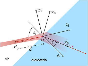
Figure 1. The figure shows the refraction of the input beam after it reaches the interface of the optical component. The propagation path of the beam is illustrated with the solid red arrow, while the dashed arrow depicting the propagation of the local plane wave  before and after the refraction. The direction of propagation of the local plane wave is slightly different from that of the beam. Geometrical alignment of incidence coordinates
  and refraction coordinates
  are shown. In the figure, the
  - and
- and  - axes point outward from the paper. The focal point of the beam is at point P, where d is the length from P to O.
Download figure:
Standard image High-resolution imageIn the figure, we define two local coordinate systems: incidence coordinates  and refraction coordinates
  . These two coordinate systems share the same origin, at point O, at which the center of the beam hits the interface. For the incidence coordinates, we assign the
  -axis and the
  -axis to be parallel and perpendicular to the plane of incidence respectively. The
  -axis, on the other hand, is defined to coincide with the direction of propagation of the incident beam. The angle between the normal vector
  and the
  -axis then gives the angle of incidence. For the refraction coordinates, we define it in such a way that the
  -axis points in the same direction as the
  -axis, while the directions of the other two axes,
  - and
- and  -axes, are given by a clockwise rotation of the
  - and
- and  -axes about the
  -axis through an angle of
  . The coordinate transformation is given by


The incident beam in a LG mode can be expressed as the superposition given in (6). We assume that the beam waist of the incident beam is located at point P on the  -axis with the distance d from the origin. Next, we consider a local plane wave component of the superposition whose wave vector expressed in the incidence coordinates
  as
as  . Notice that the propagation direction of the local plane wave is slightly different from that of the incident beam. The form of this local plane wave in the incidence coordinates can be written as
where  is the terms in the curly bracket of (7) which is the unit polarization vector of the local plane wave. The refraction of this local plane wave is described by the boundary conditions and Snell's law. We note here that each local plane wave in the superposition in (6) has its own plane of incidence, which may be slightly different from the plane of incidence of the beam itself. The local plane of incidence of the local plane wave
  is defined to be the plane that the local wave vector
  and the normal vector
  lie in. The refraction of the local plane wave
  at the interface gives rise a refracted plane wave inside the dielectric. The wave vector of the refracted plane wave is determined by using Snell's law and the fact that the frequency of an electromagnetic wave is not changed by refraction as [12]
Applying the Taylor expansion around  up to the second order, the wave vector of the refracted plane wave in the refraction coordinates
  can be expressed as
The second order of the wave vector component in the  -direction can be neglected, as in the paraxial limit its contribution to the final result is very small compared to the other mentioned terms. We then can write the refracted plane wave in terms of the refraction coordinates
  as
as

with

where  and
and  are defined to be unit vectors perpendicular and parallel to the local plane of incidence respectively, satisfying
  , and
, and  and
and  are the transmission coefficients for s-polarized and p-polarized light. In (12), we have defined
  . We note here that
  and
and  are functions of kx and ky as they depend on the angle of incidence of the local plane wave
  . The unnormalized vector
  is proportional to the polarization of the refracted plane wave. The superposition of all refracted plane waves gives us the form of the refracted beam
where  is the spatial distribution of the refracted beam. In the above equation we have used Leibniz integral rule, so the polynomials of kx and ky are replaced by the derivative operators
  and
and  respectively, which makes the vector
  become a differential operator. The spatial function of the refracted beam can be written as

with the function  defined as
where  and
and  are the beam parameters for the transverse dimensions of the refracted beam, and they can be expressed as

with q(d) is the beam parameter of the incident beam, given in (3), at the refraction point, point O. As the beam parameters for the transverse dimensions parallel and perpendicular to the plane of incidence, qx and qy, develop differently after the refraction, it means the stigmatic beam becomes astigmatic right after it is refracted with a nonzero angle of incidence. As mentioned, we are only interested in the orbital angular momentum of the refracted beam. In paraxial limit, it is solely described by the spatial distribution  , not the polarization vector of the beam. Therefore, in this work, it is no need to determine the explicit expression of the polarization.
3.2. Total internal reflection
For some optical elements, such as Dove prisms, they force the light beam to undergo total internal reflection in order to traversing through them. We assume that after the first refraction the optical beam then continuously propagates inside the medium and experiences total internal reflection, as shown in figure 2. The previously-discussed refracted beam now becomes the incident beam for the reflection with θ1 being the angle of incidence. The coordinates  shown in the figure are the same coordinates defined previously in figure 1. For simplicity's sake, we also assume that the plane of incidence of the total internal reflection is identical to that of the first refraction. We then define another coordinates
  such that the
  -axis coincides with the propagation direction of the beam after it is reflected from the interface. The
  - and
- and  -axes are assigned to be parallel and perpendicular to the plane of incidence. The axes of the coordinates
  are obtained by rotating the refraction coordinates
  about the
  -axis counterclockwise through an angle of π − 2θ1. The origin of the reflection coordinates
  is at the location where the center of the beam hits the interface. We note here that the origin of the refraction coordinates
  is at point O, displayed in figure 1. The transformation between the two coordinate systems read

Figure 2. The optical beam experiences the total internal reflection after entering the medium from point O in figure 1. The alignment of the coordinates  and
and  is shown. The
  - and
- and  -axes point outward from the paper. We note here that the coordinates
  is the refraction coordinates defined in figure 1.
Download figure:
Standard image High-resolution image

where b0 is the distance between the origin of the two coordinate systems or the distance the beam travels before reaching the reflection interface. The refracted plane wave  given in (12) now becomes the incident plane wave for this case. We can use the law of reflection to calculate the relation between the wave vector
  of the refracted plane wave
  and that of the corresponding plane wave reflected from the interface as [23]

where  is the wave vector of the reflected plane wave and
  is a unit vector normal to the surface of reflection as displayed in the figure. With the expression of
  in the refraction coordinates
  given in (11), the wave vector of the reflected plane wave written in the reflection coordinates
  becomes

Comparing this equation with (11), we notice that, when the beam experiences total internal reflection, the transverse component of the wave vector in the  -direction, which is parallel to the plane of incidence, changes its sign. This means the forms of the beam's spatial distributions
  before and after the total internal reflection are almost the same except the sign of the transverse coordinate parallel to the plane of incidence, the
  -coordinate in this case. Thus, the spatial distribution
  of the reflected beam can be expressed in the reflection coordinates
  as
as

where the function  is given in (15). This indicates that the total internal reflection changes the sign of the topological charge of the beam into the opposite. More detailed information of this is given in [23].
In general, a light beam may experience more than one total internal reflection while traveling within an optical element. For example, a Fresnel rhomb makes use of two total internal reflections to introduce π/2 phase difference between the two orthogonal components of polarization [31]. In this work, we consider only the case when all planes of incidence of all total internal reflections are parallel to each other and also to that of the first refraction.
3.3. Second refraction
Our aim now is to determine the form of the beam after it departs the medium. In figure 3, we assign point  to be the point where the center of the beam strikes the interface surface and gives rise the second refraction. We assume that the planes of incidence at the entrance point, point O, and the exit point, point
  , are parallel to each other. In other words, we simply limit our study to the case that all planes of incidence are parallel to each other while the beam traversing through the optical element. We define two coordinate systems
  and
and  such that they share the same origin, located at
  , the
, the  - and
- and  -axes are parallel to the plane of incidence, and the
  - and
- and  -axes are the propagation directions of the beam before and after it leaves the dielectric. While the beam propagating along the way to the exit point,
  , we assume that the beam has experienced N total internal reflections.
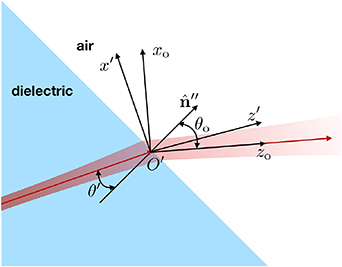
Figure 3. The second refraction of the beam occurs when the beam leaves the optical element. The alignment of the two coordinate systems  and
and  is displayed. The angles of incidence and refraction in this case denoted by
  and
and  .
.
Download figure:
Standard image High-resolution imageBefore we going further, let us summarize the previous discussion. We have considered the plane wave component  of the superposition in (6). After the first refraction, the plane wave
  gives rise to the refracted plane wave
  as shown in (12). At this point, we now assume that, as the beam propagating inside the medium, it undergoes N total internal reflections, which makes the transverse x component of the wave vector change the sign for N times. The phase of the plane wave, on the other hand, also increases while propagating inside the medium. We then obtain the form of the plane wave before reaching the exit point, point
  , written in the coordinates
  as
as

where  is an unnormalised vector pointing in the same direction as the polarization unit vector of the plane wave and L is the distance that the beam uses to travel inside the medium before the second refraction, the distance for propagating from O to
  . The last three exponentials represent the phase that the plane wave acquires before reaching the exit point,
  . When the plane wave is refracted and leaves the medium, the wave vector of the transmitted plane wave can be calculated by using Snell's law in the same manner mentioned previously in (10). The wave vector of the outgoing plane wave in the coordinates
  can be expressed as

where  and
and  are the angle of incidence and the angle of refraction for the second refraction, as depicted in the figure. The expression of the outgoing plane wave in the coordinates
  is given by

where  and
and  is a vector proportional to the polarization unit vector of the outgoing local plane wave. As previously mentioned,
  is not related to the orbital angular momentum of the beam in the paraxial limit, so its explicit form is not required in this work. We then calculate the superposition of all outgoing local plane wave to determine the form of the outgoing beam in the coordinates
  , which is

with
where the function  is defined as

with the beam parameters given by
where the definitions of qx and qy are given in (17a) and (17b).
The analogy of the forms of the beam parameters shown in the above equations and in (17a) and (17b) can be used to form the law of transformation for the beam parameters of an optical beam refracting at a flat surface as follows. For the transverse dimension parallel to the plane of incidence, the transformation of the beam parameter, denoted by qx and  , is given by the summation of the two distinct terms: 1.) the distance along the propagation direction from the refraction point, which is
  for the first refraction and
  for the second refraction, 2.) the previous beam parameter before the refraction with the relative refractive index and the square of the ratio of the cosines of the angle of refraction and the angle of incidence being the multipliers. For the other transverse dimension, the transformation is less complicated as it is just the summation of the distance from the refraction point and the product between the relative refractive index and the previous beam parameter.
At this point, we can see that unless the ratios of cosines,  and
and  , are unity, the beam parameters for different transverse dimensions are not equal to each other,
  , after the light beam leaves the medium. This indicates that the stigmatic beam is transformed into astigmatic light.
4. OAM decomposition of the outgoing beam
In the previous section, we have shown how the refraction and reflection change the form of the spatial distribution uk,l of the input LG beam. In order to understand the effect of astigmatism induced by refractions on the orbital angular momentum of the beam, in this section, we aim to analyze the change of the beam's OAM after the beam has left the medium.
Let us consider the spatial distribution given in (2), when the beam is in a pure spiral harmonic mode with the topological charge l, and compare it with the spatial distribution of the output beam  given in (26). We can see clearly that, with a nonzero angle of incidence, the spatial distribution function
  of the output beam is no longer in a form of a pure LG mode. Indeed, it is a superposition of spiral harmonic modes instead as given by [11]

with
is the coefficient of a harmonic mode with an integer topological charge m, while the relation between the cylindrical and Cartesian coordinates is described by  and
and  , where ρ and φ are the radial and azimuthal coordinates. The weight of the m-harmonic mode in the superposition can be obtained by
  . The weight Cm can also be interpreted as the probability of detecting the output photons having an orbital angular momentum of ћm.
Recall that, in the previous section, we assume the total internal reflections occur for N times while the beam propagating inside the medium. In the case that N is an even number, the weight Cm can be written as [10, 11]
with

when  is an integer and
  otherwise. The second summation of (31) run over the set
  , which is denoted to be a set of all possible pairs of non-nagative integers j1 and j2 that satisfy
  and
and  . In (33), we use Jn to represent the Bessel function of the first kind and order n with its argument s defined as

Even though the integrand in (31) depends on  , the weights of the harmonic modes themselves do not change while the beam propagating in free space [11, 32], due to the conservation of angular momentum. The summation over all weights Cm satisfies
  . On the other hand, if the number of the total internal reflections, N, is an odd number, we replace the term
  in (33) with
  to obtain the weights Cm. We note here that, with the currently available technology, the coefficients am and the weights Cm can be measured experimentally [32]. In order to see how these equations describe the OAM decomposition of the output beam, we consider the following given examples.
From above equations, we can see that, if we let a LG beam with an orbital angular momentum of ћl per photon passes through a dielectric slab at normal incidence,  , the output beam is still stigmatic as the beam parameters for both transverse dimensions are equal to each other
  . This makes
  , where δi,j is the Kronecker delta. We note here that a stigmatic beam is always in a pure spiral harmonic mode. This means the OAM decomposition of the light beam is preserved. The probability of finding the orbital angular momentum per photon ends up in any values other than ћl is zero.
In figure 4, we display the geometries of the dielectric slab and the Dove prism together with the optical paths of the light beams governed by Snell's law. The ratios of the cosines of the angles of incidence and refraction at the entrance and exit points are the multiplicative inverses of each other, i.e.  , which gives
  . Applying this to (28a) and (28b), it indicates that the beam waist positions of the output beam for both transverse directions differ from each other by
  . We then consider the case when the Rayleigh length
  of the incident beam is much larger than the dimensions of the dielectric slab and the Dove prism, so that
  . Otherwise speaking, this is the case when the difference between the beam waist positions for the different transverse directions is small compared to the Rayleigh length. The beam is almost stigmatic. We find that, if the incident beam is in an l-harmonic mode at the beginning, after it passes through the dielectric slab (Dove prism), the weight of the l-harmonic mode (−l-harmonic mode) is approximately unity, Cl≈ 1 (C−l≈ 1). In other words, the probability of finding the output beam having ћl (−ћl) orbital angular momentum per photon is close to 1.
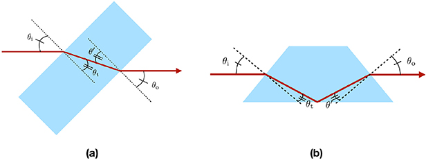
Figure 4. The optical paths of the beams propagating in (a) the dielectric slab and (b) the Dove prism are illustrated with solid red lines. The geometries of the optical paths indicate that  .
.
Download figure:
Standard image High-resolution image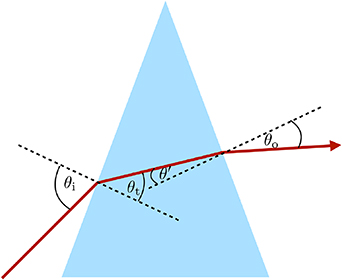
Figure 5. The picture shows the optical path of the light beam in a dispersive prism. In contrast to the cases of dielectric slabs and Dove prisms, the ratios of cosines at the entrance and exit points do not have to be the inverses of each other, which means it is not necessary that  in this case.
Download figure:
Standard image High-resolution imageIt becomes a different story when the sizes of these two optical elements are comparable to the Rayleigh length. We note that the paraxial approximation is still valid for this case. For example, a beam with wave length λ = 600 nm and the waist radius w0 = 40 µm is still in the paraxial regime [33]. The Rayleigh length of this beam is 8.4 mm which is comparable to or even smaller than the usual sizes of dielectric slabs and Dove prisms. In this case, the astigmatism significantly changes the OAM decomposition of the beam as demonstrated in figure 6. In the figure, it shows the OAM decompositions of the out beam before and after the second refraction, given that the incident beam is in a LG mode with l = 1. The light beam is assumed to pass through the dielectric slab (the Dove prism) in such a way that  and
and  . The OAM decompositions before and after the beam leaves the dielectric slab (the Dove prism) is displayed in the first (second) row of the figure. By comparing the first and second columns in the first two rows, we can notice that before and after the second refraction the weights Cm of the orbital angular momentum distribute around m = l or m =−l differently, and the reason is as follows. The first refraction modifies the Rayleigh lengths for both transverse dimensions unequally:
  , where
  is the Rayleigh length for the ith dimension. We find that the ratio of the magnitude of the Minkowski-type orbital angular momentum (see the definition in [34, 35]), denoted by Lz, to the energy density
  of the refracted beam is larger than that of the initial beam:
  . This leads to the asymmetric distribution of Cm. As
  , the second refraction, on the other hand, equalizes the Rayleigh lengths, i.e.
  , which makes the distributions of Cm after the second refraction are symmetric around m = l or m =−l. However, the second refraction also modifies the beam waist positions for different transverse dimensions differently as mentioned. Because of the total internal reflection at the base of the Dove prism, the signs of the orbital angular momentum after traversing through the Dove prism and the dielectric slab are different. From the figure, the probability that the Dove prism changes the orbital angular momentum per photon from ћl to −ћ(l + 2) or −ћ(l − 2) instead of −ћl is no longer negligible. The phase profiles of the output beams after transversing through the dielectric slab and the Dove prism are shown in figure 7. They are mirror images of each other. As shown in the figure, the rates at which the azimuthal phases φ of the output beams grow from 0 to 2π differ from that of the initial beam. They grow from 3π/4 to 5π/4 slightly slower, while changing from π/4 to 3π/4 and from 5π/4 to 7π/4 quicker.

Figure 6. The distributions of the weights Cm are displayed. The incident beam is in a LG mode with l = 1. The first column shows the distributions of Cm before the second refraction, while the second column illustrates the weight distributions after the second refraction. In the figure, each row is dedicated to each optical element. We assume that the optical paths of the beams inside the dielectric slab and the Dove prism satisfy  and
and  . On the other hand, the light beam is supposed to pass through the dispersive prism in such a way that
  , while the optical path inside the dispersive prism is very small compared to the Rayleigh length:
  .
.
Download figure:
Standard image High-resolution image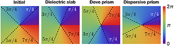
Figure 7. The figure shows the phase profiles of the initial beam and those of the beams after traversing through the dielectric slab, the Dove prism and the dispersive prism. The dashed lines mark the positions at which the azimuthal phase φ equal to π/4, 3π/4, 5π/4 and 7π/4.
Download figure:
Standard image High-resolution image
Equilateral dispersive prisms, on the other hand, are generally used in various purposes in experimental setups such as changing the beam direction or controlling the dispersion [36]. From the optical path shown in figure 5, we find that, in general, unlike the previous case, the ratios of cosines may not cancel out each other, which gives  . The OAM decomposition of the beam after traversing through a prism is changed remarkably, even though the optical path L inside the medium is very small compared to the Rayleigh length
  of the input beam. In figure 6, we provide the OAM decomposition for the output beam after it traveling through the dispersive prism, given again that the input beam is in a LG mode with l = 1. We consider the case when
  and
and  . The weights Cm of the OAM superposition are asymmetrically distributed around m = l. As mention, the asymmetric distribution of Cm arises because the Rayleigh lengths in different transverse dimensions are unequal,
  . In figure 7, the phase profile of the beam after traveling through the dispersive prism is displayed. It is considerably different from those in the previous cases. The azimuthal phase of the output beam grows from 3π/4 to 5π/4 quicker than that of the initial beam, while it changes from π/4 to 3π/4 and from 5π/4 to 7π/4 distinctively slower. We note that, in the minimum-deviation configuration of the light beam, i.e.
  , the distribution of the OAM decomposition of the output beam is symmetric around m = l in the same way as the case of the dielectric slab.
At this point, we can summarize that astigmatism caused by refraction changes the OAM decomposition of the beam. Without awareness of its effect, the undesired transformation of the OAM state can introduce errors to the realization of the quantum algorithms and protocols that make use of Dove prisms and dispersive prisms, to manipulate the OAM state of photons or to change the propagation direction. The compensation scheme or error correction is required.
5. Conclusion
We have demonstrated theoretically, with wave optics, that refraction with non-zero angles of incidence can induce astigmatism to a stigmatic OAM beam. Each refraction makes the beam parameters for the two orthogonal transverse dimensions develop differently along the propagation path of the beam. This effect transforms a well-defined OAM state of photons into a superposition of OAM states after refraction.
Acknowledgments
The author would like to thank Stephen M. Barnett for useful suggestion and discussion. I acknowledge financial support from the Development and Promotion of Science and Technology Talents Project (DPST), Thailand.