Efficient 3D trilateration algorithm for visible light positioning

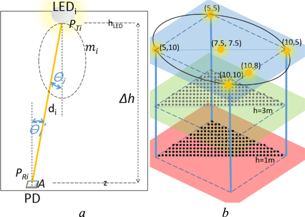
We assume a generic configuration with N LEDs, each horizontally placed at a fixed height h_LED, denoted with LED_i and with coordinates (x_i, y_i, h_LED), i = 1 .. N. The Lambertian mode of LED_i is denoted as m_i and its transmitted power as P_Ti. The PD, with area A, is also horizontally oriented and located at the unknown location (x, y, z) at an unknown distance d_i from LED_i. The angle of irradiance is defined as θ_i and the angle of incidence as ${\theta }_{i}^{{\prime} },$ as shown in figure 1(a). A setup with four LEDs in a 5 × 5 × 5 m³ volume is considered; see figure 1(b). According to the channel model of [5], the power P_Ri received from LED_i, at (x, y, z) is given by:

$$\begin{eqnarray}&&{{P}}_{{Ri}}={\cos }^{{m}_{i}}\left({\theta }_{i}\right)\,\cos \left({\theta }_{i}^{{\prime} }\right)\,\left({m}_{i}+1\right)\,{A}\,\displaystyle \frac{{{P}}_{{Ti}}}{2\,\pi {d}_{i}^{2}}.\end{eqnarray} \tag{ 1 }$$

Zoom In Zoom Out Reset image size

Inversely, given a measured power P_Ri received at an unknown location, and knowing $\cos \left({\theta }_{i}\right)=\,\cos \left({\theta }_{i}^{{\prime} }\right)=\tfrac{{{h}}_{{\rm{LED}}}-z}{{d}_{i}}$ for horizontally oriented LEDs and PD (see figure 1(a)), the distance d_i between the PD and LED_i can be estimated as ${\widehat{d}}_{i},$ based on the power P_Ri received from LED_i (i = 1 .. N):

$$\begin{eqnarray}&&{\hat{d}}_{i}=\sqrt[{m}_{i}+3]{\displaystyle \frac{\left({m}_{i}+1\right)\,A\,{P}_{Ti}\,{\rm{\Delta }}{h}^{{m}_{i}+1}}{2\,\pi \,{P}_{Ri}}}\end{eqnarray} \tag{ 2 }$$

with Δh = h_LED−z = the (unknown) height difference between LED_i and the PD. As such, ${\widehat{d}}_{i}$ cannot be directly determined from P_Ri, due to the angle-dependent behavior of the transmitter: locations at different distances from the transmitter (and at different heights) might lead to the same P_Ri measurement. Therefore, a classic trilateration algorithm cannot be straightforwardly applied. In the following, we will denote ${\widehat{d}}_{i}$ as ${\widehat{d}}_{i}$ (Δh), due to its height dependency.

The proposed algorithm is based on an iterative 2D trilateration combined with a nonlinear least squares (NLLS) minimization to find the most likely 3D location. Both parts will be explained hereafter.

2D trilateration—since the distances d_i cannot be estimated directly, we can only use a 2D trilateration at an assumed Δh, for N LED sources. The squared horizontal distance between LED_i and the PD is given by:

$$\begin{eqnarray*}\begin{array}{lll}{d}_{i}^{2}\left({\rm{\Delta }}h\right) & = & {\left(x-{x}_{i}\right)}^{2}+{\left(y-{y}_{i}\right)}^{2}\\ & = & {x}^{2}-2x{x}_{i}+{x}_{i}^{2}+{y}^{2}-2y{y}_{i}+{y}_{i}^{2}.\end{array}\end{eqnarray*}$$

After eliminating the quadratic terms in x² and y² by subtracting ${d}_{N}^{2}$ from ${d}_{i}^{2},$ N − 1 equations are obtained (i = 1 .. N − 1):

$$\begin{eqnarray*}\begin{array}{lll}{d}_{i}^{2}\left({\rm{\Delta }}h\right)-{d}_{N}^{2}\left({\rm{\Delta }}h\right) & = & -2x\left({x}_{i}-{x}_{N}\right)+{x}_{i}^{2}-\,{x}_{N}^{2}\\ & & \,-\,2y\left({y}_{i}-{y}_{N}\right)+{y}_{i}^{2}-{y}_{N}^{2}.\end{array}\end{eqnarray*}$$

These linear equations in x and y can be written as ${\boldsymbol{b}}={\boldsymbol{A}}\left[\begin{array}{c}x\\ y\end{array}\right],$ where

$$\begin{eqnarray}&&{\boldsymbol{b}}=\left[\begin{array}{c}{d}_{1}^{2}\left({\rm{\Delta }}h\right)-{x}_{1}^{2}-{y}_{1}^{2}-{d}_{N}^{2}\left({\rm{\Delta }}h\right)+{x}_{N}^{2}+{y}_{N}^{2}\\ {d}_{2}^{2}\left({\rm{\Delta }}h\right)-{x}_{2}^{2}-{y}_{2}^{2}-{d}_{N}^{2}\left({\rm{\Delta }}h\right)+{x}_{N}^{2}+{y}_{N}^{2}\\ \vdots \\ {d}_{N-1}^{2}\left({\rm{\Delta }}h\right)-{x}_{N-1}^{2}-{y}_{N-1}^{2}-{d}_{N}^{2}\left({\rm{\Delta }}h\right)+{x}_{N}^{2}+{y}_{N}^{2}\end{array}\right],\end{eqnarray} \tag{ 3 }$$

$$\begin{eqnarray}{\boldsymbol{A}}=-2\left[\begin{array}{cc}{x}_{1}-{x}_{N} & {y}_{1}-{y}_{N}\\ {x}_{2}-{x}_{N} & {y}_{2}-{y}_{N}\\ \vdots & \vdots \\ {x}_{N-1}-{x}_{N} & {y}_{N-1}-{y}_{N}\end{array}\right].\end{eqnarray} \tag{ 4 }$$

For any given Δh, $\left[\begin{array}{c}x\\ y\end{array}\right]$ can then be estimated as $\left[\begin{array}{c}\hat{x}\\ \hat{y}\end{array}\right],$ using the Moore–Penrose pseudo-inverse of A:

$$\begin{eqnarray}&&\left[\begin{array}{c}\hat{x}\left({\rm{\Delta }}h\right)\\ \hat{y}\left({\rm{\Delta }}h\right)\end{array}\right]={\left({{\boldsymbol{A}}}^{{\boldsymbol{T}}}{\boldsymbol{A}}\right)}^{-1}{{\boldsymbol{A}}}^{{\boldsymbol{T}}}{\boldsymbol{b}}.\end{eqnarray} \tag{ 5 }$$

NLLS optimization—in this phase, the 2D trilateration process is repeated for each of the candidate heights h, varying between a minimum height h_min and maximal height h_max < h_LED, with a height resolution R_h. The estimated location is found at the minimum of C(h), which is defined as the average squared error between the estimated distances ${\hat{d}}_{i}$ (h) from (2) and the distances of the estimated location ($\hat{x}$(h), $\hat{y}$(h), h) from (5) [6]. It determines to what extent the assumed height h when performing the trilateration, was likely

$$\begin{eqnarray}&&\begin{array}{l}C\left(h\right)=\displaystyle \frac{1}{N}\displaystyle \sum _{i=1}^{N}\left[\widehat{{d}_{i}}\left(h\right)\right.\\ \,\,\,-{\left.\sqrt{{\left(\hat{x}(h)-{x}_{i}\right)}^{2}+{\left(\hat{y}(h)-{y}_{i}\right)}^{2}+{\left(h-{z}_{i}\right)}^{2}}\right]}^{2}.\end{array}\end{eqnarray} \tag{ 6 }$$

Algorithm 1. Summarizes the iterative trilateration approach with NLLS.

Algorithm 1 Iterative trilateration algorithm with NLLS

In: measured PRi values, A, mi, PTi, and LED settings (see table 1)

Out: estimated location locest(x, y, z)

1. Initialization: Costmin = max_value, locest = null

2. for (h = hmin: Rh: hmax)

3. Δh = hLED-h

4. calculate ${\hat{d}}_{i}$ (Δh) based on (2) for i = 1 .. N

5. calculate $\left[\begin{array}{c}\hat{x}({\rm{\Delta }}h)\\ \hat{y}({\rm{\Delta }}h)\end{array}\right]$ based on the insertion of ${\hat{d}}_{i}$ (Δh) in (5)

6. calculate cost function C(h) of (6) and update Costmin: if (C(h) < Costmin)

Costmin = C(h); locest = ($\hat{x}\left({\rm{\Delta }}h\right),$ $\hat{y}\left({\rm{\Delta }}h\right)\,,$ h)

end if

7. end for

The algorithm performance is first evaluated for the LED configurations denoted as CFG1 to 4 in table 1. The PD height is set to 1 m (see figure 1(b)) with A = 1 mm². The LEDs are mounted at h_LED = 5 m, with a transmitted power of 10 W each, and m = 1 (except LED₄ in CFG4). Candidate heights vary between 0 and 4 m, with a resolution R_h = 1 mm.

Without noise added to the P_Ri values of (1), it is observed that with three LEDs (CFG1), there are always two possible 3D solutions for the receiver. Figure 2 shows the cost function C(h) for location (5.5, 7.5, 1), becoming zero at h = 1 m, but also at h = 2.5 m, leading to the location (6.25, 7.5, 2.5). Adding a fourth LED (with the same P_T and m) is able to solve this ambiguity, provided that is not located on the circle formed by the first three LEDs (see figure 1(b)), which is due to the radiation pattern's geometrical properties. Figure 2 shows that C(h) for CFG1 is the same as for CFG2 (curves overlap). It can indeed be calculated with (1) that the received powers at the two locations are the same in CFG2, i.e. (P_R1, P_R2, P_R3, P_R4) (nW) = (101, 28, 101, 28). As such, the traditional much-used square-shaped LED configuration with 4 LEDs on a circle (CFG2) is not preferred, as the fourth LED has no added value compared to CFG1 with 3 LEDs. Adding a LED that is not located on circles formed by other LED combinations (e.g. LED₄ in CFG3), eliminates the second minimum at h = 2.5 m, as shown in figure 2. A second way of resolving the location ambiguity of CFG1, is mounting a fourth LED on the circle, but with a different mode m. Figure 2 indeed shows a unique minimum of C(h) at h = 1 m in CFG4 (with LED₄ on the circle, but with m = 3). However, an LED configuration with different m values for different LEDs is usually not preferred in view of lighting conditions. The aforementioned analysis is valid for any 3D PD location.

Zoom In Zoom Out Reset image size

After showing the proper operation of the 3D trilateration algorithm, we now investigate the performance when Gaussian noise with a standard deviation of 1 nW is added to the idealized P_Ri values of (1). Per height level, 1301 points inside the LED triangle formed by LED_1–2–3 are evaluated on a uniform grid of 10 cm (see figure 1(b)), in CFG1, CFG3, and CFG5 (using 3, 4, and 5 LEDs, respectively). For each of the locations, five simulations are done with random noise levels and using R_h = 1 cm.

Figure 3 shows the cumulative distribution function (cdf) of the positioning errors for CFG1-3-5. At h = 1 m and for CFG1 (3 LEDs), it can be seen that slightly less than 60% of the points is clustered around the correct location with errors below 50 cm, and the rest around the equally likely alternatives having errors up to 3 m. For CFG3 (4 LEDs) and CFG5 (5 LEDs), median errors decrease (from 18.7 cm to 7.3 and 4.8 cm respectively), a.o. because there is only one cost minimum (see figure 2). For h = 3 m and CFG1, the error ranges of the two clusters overlap, making a smoother curve compared to h = 1 m. Errors at h = 3 m are mostly larger than at h = 1 m, because received LED powers are lower on average, due to larger angles θ (see (1)), while assuming a same noise level. Median errors at h = 3 m equal 31.8, 9.1, and 5.8 cm for CFG1, CFG3, CFG5, respectively.

Zoom In Zoom Out Reset image size

Using MATLAB R2018a on a 2.1 GHz Intel i7 processor with 8 GB RAM, one location estimation for CFG3 takes 16.6 ms on average for a height resolution of 1 cm (401 candidate heights between 0 and 4 m). This indicates that the proposed method is able to estimate the 3D position in real-time, making it suitable for drone navigation using only a PD, for example.

Since most 3D VLP applications will rely on constrained receiver modules that are mobile, wireless, and lightweight, it is crucial to minimize calculation time (and thus power consumption) of the algorithm as much as possible. Therefore, a fast search method is added to algorithm 1. Instead of iterating uniformly over all candidate heights between h_min and h_max (see line 2 of algorithm 1), we propose an adapted version of the one-dimensional golden section search (GSS) algorithm [7]. This fast search method iteratively narrows the search interval inside which the extremum is located. Since GSS can only be applied to unimodal functions and C(h) can possibly be bimodal (see e.g. CFG3 in figure 2), we first coarsely determine the interval inside which the lowest minimum is located, by evaluating C(h) at candidate heights within the interval [h_min, h_max], with a resolution of 30 cm, as it is observed that location ambiguity occurs for PD heights spaced more than 30 cm apart. The height h producing the minimal C(h) value over this sparse search set is defined as h*, i.e. $h* =\text{arg}\mathop{\,\min }\limits_{h}{C}\left(h\right).$ Then, the regular GSS algorithm is applied to the interval $\left[{h}_{{\min }}^{{\rm{G}}{\rm{S}}{\rm{S}}},{{h}}_{{\max }}^{{\rm{GSS}}}\right],$ with ${{h}}_{{\min }}^{{\rm{GSS}}}=h* -30\,{\rm{cm}},$ and ${{h}}_{{\max }}^{{\rm{GSS}}}=h* +30\,{\rm{cm}},$ capped at h_min and h_max, respectively. The GSS algorithm is terminated when the search interval is less than 1 cm wide, in order to get a same height resolution R_h as in the original algorithm 1. The estimated PD height is set as the average of the final interval's bounds and (x, y) is estimated with the classic 2D trilateration (lines 4 and 5 of algorithm 1).

Figure 3 shows that for a same configuration (i.e. CFG3 evaluated at h = 1 m), this efficiency-optimized algorithm produces the same error cdf as the non-optimized version. However, besides maintaining the positioning performance, it reduces the average execution time over the receiver grid by 90%, from 16.6 to 1.7 ms per 3D position estimation. For real-life deployments, the execution time can possibly be further reduced, by narrowing the initial [h_min, h_max] interval, i.e. with bounds determined by the previous PD height, the maximal vertical PD speed and the location update rate.