Position correction in ptychography using hybrid input–output (HIO) and cross-correlation

Computationally imaging an object—replacing lenses with algorithms—is becoming extremely popular. Over the years, several iterative algorithms have been developed including the error-reduction algorithm [1], the hybrid input–output (HIO) algorithm [2], the hybrid projection-reflection algorithm [3], the relaxed averaged alternating reflectors (RAAR) algorithm [4]. These methods reconstruct an object from a single intensity pattern. An algorithm called ptychographic iterative engine (PIE) [5] was developed, which uses several intensity patterns for reconstruction and was found to be superior to other existing methods.

In ptychography, an object is scanned by a localised probe in a way that the neighbouring probe positions should overlap with each other; corresponding to these probe positions, the diffraction patterns are captured in the far-field. These diffraction patterns are employed to reconstruct the complex object. The crucial aspect for the success of this method is the overlap between neighbouring probe positions. The optimum overlap has been found to be about 60% [6].

Ptychography has given significant results with visible light experiments [7], whereas the reconstructions have suffered for x-rays and e-beams data—the limitations were due to the inaccurately known initial parameters, e.g. probe positions [8, 9]. The illuminating probe function, for instance, should be known accurately. To this end, extended PIE has been introduced to eliminate the requirement of accurately known probe function [10]. Later on, it was found that probe positions for electron ptychography should be known with an accuracy of 50 pm [11], which is difficult to achieve experimentally. Several successful attempts, subsequently, have been made to solve the probe positions correction problem.

For example, one finds in the literature the 'annealing approach' based on 'trial and error', but this is computationally expensive [12]. In yet another study, nonlinear (NL) optimisation with ePIE is used [13]. NL optimisation, however, can not correct with sub-pixel accuracy. To achieve this, one is required to use the cross-correlation (CC) method [11], which has been widely used. Recently, we have proposed a new method based on gradient of intensity patterns [14] that can correct the probe positions with sub-pixel accuracy while being less computationally expensive than the CC method.

In this work, we introduce a novel method for the correction of the probe positions in ptychography [15]. This method combines the well known techniques HIO and cross-correlation in a way that it can also correct probe positions in ptychography. This is possible mainly due to two important properties:

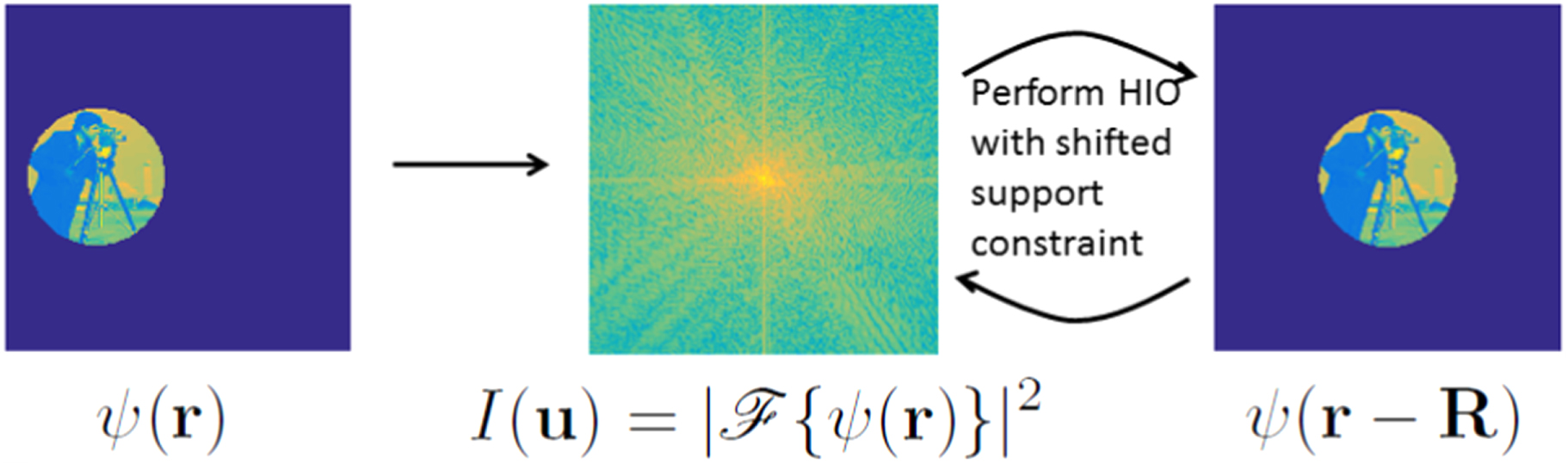
• The reconstructed object using single intensity method is indifferent to wrong/shifted support constraint, except, the reconstructed object is shifted laterally as shown in figure 1.
• Sufficient overlap between neighbouring probe positions gives information about the relative shift between neighbouring probe positions. If the probe positions were correct, the overlapped part of the object corresponding to neighbouring probe positions will coincide with each other (see figure 2).

The performance of this method with varying parameters and its limitations are presented here. The paper is organised as follows: in section 2, we elaborate on the new method in detail. Section 3 details the simulation results to asses its performance. In section 4, we discuss the main findings and its limitations. Finally, we present the conclusions in section 5.

Zoom In Zoom Out Reset image size

Zoom In Zoom Out Reset image size

In ptychography, an object $O({\bf{r}})$ is scanned by a probe/aperture $P({\bf{r}}-{{\bf{R}}}^{j})$ and the corresponding intensity patterns ${I}^{j}({\bf{u}})$ are captured in the far-field. Here ${\bf{r}}$ and ${\bf{u}}$ are the coordinate vectors in the real and the reciprocal space, respectively. ${{\bf{R}}}^{j}$ is the $j\mathrm{th}$ probe position vector. If J is the total number of probe positions, j = 1, 2, 3 ... J.

From the property of the Fourier transform, translating a wave-field along the x or y axis in real space does not affect the intensity pattern in the far-field. Therefore, for a single-intensity phase retrieval method, the reconstruction of the object will be indifferent to the position of the support constraint except that the reconstructed object will be at a different place in the real space. In figure 1, the exit wave $\psi ({\bf{r}})=O({\bf{r}})P({\bf{r}})$, the intensity pattern in the far-field, and the reconstruction with shifted support constraint $P({\bf{r}}-{\bf{R}})$ are shown. Here, the reconstruction was performed using HIO.

Now, let us assume that the probe positions in ptychography are not accurately known. If we reconstruct the exit wave ${\psi }^{j}({\bf{r}})$ defined by the probe $P({\bf{r}}-{{\bf{R}}}^{j})$ using HIO and find the part of the object ${O}^{j}({\bf{r}})$ corresponding to ${\psi }^{j}({\bf{r}})$, we will have the correct part of the object at a wrong probe position. This will create a miss-match in the overlapped region between parts of the object ${O}^{j-1}({\bf{r}})$ and ${O}^{j}({\bf{r}})$ which correspond to neighbouring probe positions. Hence, by finding the maxima of their cross-correlation, one can find the relative shift between neighbouring probe positions. In figure 2, the overlapped region of ${O}^{j-1}({\bf{r}})$ and ${O}^{j}({\bf{r}})$ are shown. In figure 2(a), the probe positions are known accurately; in figure 2(b), the estimated probe positions have an error.

The proposed algorithm is a sequential combination of ePIE, HIO and cross-correlation. For the kth iteration, the steps of the algorithm are as follows:

• 1.  
  Perform a few iterations (say l) of ePIE with the estimated object ${O}_{k}({\bf{r}})$, the probe ${P}_{k}({\bf{r}})$ and the probe positions ${\left\{{{\bf{R}}}_{k}^{j}\right\}}_{j=1}^{J}$ to obtain a better estimate of the object ${O}_{k}^{{\prime} }({\bf{r}})$ and the probe ${P}_{k}^{{\prime} }({\bf{r}})$.
• 2.  
  Calculate the exit wave corresponding to each probe position j as:

  $$\begin{eqnarray}&&{\psi }_{k}^{j}({\bf{r}})={O}_{k}^{{\prime} }({\bf{r}}){P}_{k}^{{\prime} }({\bf{r}}-{{\bf{R}}}_{k}^{j}).\end{eqnarray} \tag{ 1 }$$
• 3.  
  Update each exit wave ${\psi }_{k}^{j}({\bf{r}})$ separately using HIO (say m iterations) where the support constraint will be defined by the probe function ${P}_{k}^{{\prime} }({\bf{r}}-{{\bf{R}}}_{k}^{j})$.
• 4.  
  With each improved exit wave ${\psi }_{k}^{j}({\bf{r}})$, calculate the corresponding part of the object as:

  $$\begin{eqnarray}{O}_{k}^{j}({\bf{r}})=\left\{\begin{array}{ll}\displaystyle \frac{{\psi }_{k}^{j}({\bf{r}})P{{\prime} }_{k}^{* }({\bf{r}}-{{\bf{R}}}_{k}^{j})}{| {P}_{k}^{{\prime} }({\bf{r}}-{{\bf{R}}}_{k}^{j}){| }^{2}} & \mathrm{if}\ | {P}_{k}^{{\prime} }({\bf{r}}-{{\bf{R}}}_{k}^{j}){| }^{2}\geqslant \alpha \\ 0 & \mathrm{otherwise},\end{array}\right.\end{eqnarray} \tag{ 2 }$$

  where α is a small number.
• 5.  
  Calculate the overlapped region ${S}_{k}^{j}({\bf{r}})$ between neighbouring parts of the object, i.e. ${O}_{k}^{j-1}({\bf{r}})$ and ${O}_{k}^{j}({\bf{r}})$ as:

  $$\begin{eqnarray}{S}_{k}^{j}({\bf{r}})=\left\{\begin{array}{ll}1 & \mathrm{if}\ | {O}_{k}^{j-1}({\bf{r}}){O}_{k}^{j}({\bf{r}})| \geqslant \beta \\ 0 & \mathrm{otherwise},\end{array}\right.\end{eqnarray} \tag{ 3 }$$

  where β is a threshold parameter. Then, calculate the cross-correlation C as:

  $$\begin{eqnarray}&&C({\boldsymbol{\rho }})=\left|\displaystyle \sum _{{\bf{r}}}{O}_{k}^{j-1}({\bf{r}}){S}_{k}^{j}({\bf{r}}){O}_{k}^{j* }({\bf{r}}-{\boldsymbol{\rho }}){S}_{k}^{j}({\bf{r}}-{\boldsymbol{\rho }})\right|.\end{eqnarray} \tag{ 4 }$$

  Determine the vector ${\boldsymbol{\rho }}={{\boldsymbol{\rho }}}_{\max }$ for which $C({\boldsymbol{\rho }})$ is maximum, and this vector ${{\boldsymbol{\rho }}}_{\max }$ should be equal to the relative shift between neighbouring probe positions ${\rm{\Delta }}{{\bf{R}}}_{k}^{j}\equiv {{\bf{R}}}_{k}^{j}-{{\bf{R}}}_{k}^{j-1}$. Then, we update ${{\bf{R}}}_{k}^{j}$ and ${O}_{k}^{j}({\bf{r}})$ as:

  $$\begin{eqnarray}&&{{\bf{R}}}_{k+1}^{j}={{\bf{R}}}_{k}^{j}+{\rm{\Delta }}{{\bf{R}}}_{k}^{j},\end{eqnarray} \tag{ 5 }$$

  $$\begin{eqnarray}&&{O}_{k}^{j}({\bf{r}})={O}_{k}^{j}({\bf{r}}-{\rm{\Delta }}{{\bf{R}}}_{k}^{j}).\end{eqnarray} \tag{ 6 }$$

  Step 5 is performed for all the probe positions j = 1, 2, 3 ... J sequentially to find the updated probe positions ${\left\{{{\bf{R}}}_{k+1}^{j}\right\}}_{j=1}^{J}$. Note that, $j-1$ and j do not always correspond to neighbouring probe positions. Therefore, when probe position $j-1$ is not the neighbour of the probe position j, we replace $j-1$ by the neighbouring probe position. In figure 3, the shaded regions show the overlapped parts which are used for the probe positions correction.
• 6.  
  With the updated probe positions ${\left\{{{\bf{R}}}_{k+1}^{j}\right\}}_{j=1}^{J}$, obtain the updated object estimate as a weighted average of the ${\psi }_{k}^{j}$ given by:

  $$\begin{eqnarray}{O}_{k+1}({\bf{r}})=\left\{\begin{array}{lc}\displaystyle \frac{{\displaystyle \sum }_{j}{\psi }_{k}^{j}({\bf{r}}){P}_{k}^{* }({\bf{r}}-{{\bf{R}}}_{k+1}^{j})}{{\displaystyle \sum }_{j}| {P}_{k}({\bf{r}}-{{\bf{R}}}_{k+1}^{j}){| }^{2}} & \mathrm{if}\ | {P}_{k}({\bf{r}}-{{\bf{R}}}_{k+1}^{j}){| }^{2}\geqslant \alpha \\ 0 & \mathrm{otherwise},\end{array}\right.\end{eqnarray} \tag{ 7 }$$

  where α is a small number, and update the probe function by:

  $$\begin{eqnarray}&&{P}_{k+1}={P}_{k}^{{\prime} }.\end{eqnarray} \tag{ 8 }$$
• 7.  
  Go back to step 1.

Each iteration of this method contains 5–10 iterations of ePIE and 50–200 iterations of HIO for each probe position. In section 3.2, simulations are shown for varying number of HIO iterations. Since, in step 3, HIO has been used with the ${P}_{k}^{{\prime} }({\bf{r}}-{{\bf{R}}}_{k}^{j})$ as a support constraint, the proposed method has a limitation on the probe function: it should be zero outside the known defined area.

Zoom In Zoom Out Reset image size

3.1. Simulations

To assess the performance of the algorithm, we performed simulations using parameters that correspond to a visible light experiment. Let us suppose that the wavelength of the light is $\lambda =400\,\mathrm{nm};$ the focal length of the lens which was used to create the Fourier transform, is f = 10 cm; the detector has 512 × 512 pixels and the detector pixel size is ${\rm{\Delta }}{x}_{d}=10\,\mu {\rm{m}}$. The detector pixel size in x and y directions are same. Thus, the size of the pixel along the x-axis in object plane is ${\rm{\Delta }}{x}_{o}=\tfrac{\lambda f}{N{\rm{\Delta }}{x}_{d}}$. The object used in the simulations has 224 × 224 pixels. The illuminating probe was created using a pinhole of radius $67.2\,{\rm{\Delta }}{x}_{o}$ and placed 1.25 mm upstream of the object. To conform with the limitation on the probe function, the illumination function on the object plane was set to zero outside the pinhole of radius $67.2{\rm{\Delta }}{x}_{o}$. To define the probe positions, a grid of 4 × 4 was created with a grid interval of $22\,{\rm{\Delta }}{x}_{o}$. The overlap between the neighbouring probe positions was 82%. Random integer offset taken from [−5, 5] pixels was added to each probe positions; these probe positions were used to generate the intensity patterns.

'Camera Man' was used as the object amplitude varying from [0.23, 1]; 'Pirate' was used as the object phase varying from [−0.7π, 0.7π]. In the simulations, first l iterations of PIE or ePIE were performed to obtain a better object estimate. Then, m iterations of HIO were performed sequentially as explained in section 2. We call the combination—l iterations of PIE, m iterations of HIO, and position correction—as one iteration of the proposed method. During the first iteration of the proposed method, we used l = 10 iterations of PIE and m = 70 iterations of HIO. From the second iteration onwards, l = 5 iterations of ePIE and m = 70 iterations of HIO were used. The feedback parameter for HIO was 0.9. The algorithm ran 5 iterations of the proposed method.

Figures 4(a)–(d) show the object and the probe to generate the intensity patterns. Figures 4(e)–(h) are the reconstructed object and the probe when ePIE is used with incorrect probe positions. Figures 4(i)–(l) show the reconstruction of the object and the probe when the proposed method was used. We calculate the mean error of the estimated probe positions using the following expression:

$$\begin{eqnarray}&&{E}_{k}=\sqrt{{\langle {\rm{\Delta }}{X}_{k}^{j}-\overline{{\rm{\Delta }}{X}_{k}^{j}}\rangle }^{2}+{\langle {\rm{\Delta }}{Y}_{k}^{j}-\overline{{\rm{\Delta }}{Y}_{k}^{j}}\rangle }^{2}}.\end{eqnarray} \tag{ 9 }$$

Here, ${\rm{\Delta }}{X}_{k}^{j}={X}^{j}-{X}_{k}^{j}$ and ${\rm{\Delta }}{Y}_{k}^{j}={Y}^{j}-{Y}_{k}^{j}$, where $({X}^{j},{Y}^{j})={{\bf{R}}}^{j}$ is the correct probe position and $({X}_{k}^{j},{Y}_{k}^{j})={{\bf{R}}}_{k}^{j}$ is the estimated probe position at the kth iteration and the jth probe position.

Zoom In Zoom Out Reset image size

In figure 5, the plot for the rms error of the probe positions versus the iteration number are shown. Ten simulations were performed with random initial probe position errors varying from [−5, 5] pixels. The solid line shows the mean and the semi-transparent patch is the standard deviation. As can be seen, for all ten simulations, the probe positions converge to the correct values in one iteration of the proposed method. This method can correct the probe positions with integer pixel accuracy.

Zoom In Zoom Out Reset image size

3.2. Varying number of ePIE and HIO iterations

The entire point of ptychography is that the neighbouring exit waves should overlap with each other, whereas here, the exit waves are also updated separately using HIO. One can question on the added value of ptychography if the object is already being reconstructed using HIO. Hence, we performed ten simulations when ePIE was not used at all. The parameters for the simulations were the same as in section 3.1 except the number of PIE iterations l was zero. As can be seen from the figure 6, the algorithm diverges. It can be explained by the inability of HIO to converge to the correct solution. There is an equal probability for HIO to converge to the twin image of the object if the support constraint is centro-symmetric, which is the case for our simulations. Whereas, a few iterations of PIE gives a better initial estimate for HIO to converge to the correct solution.

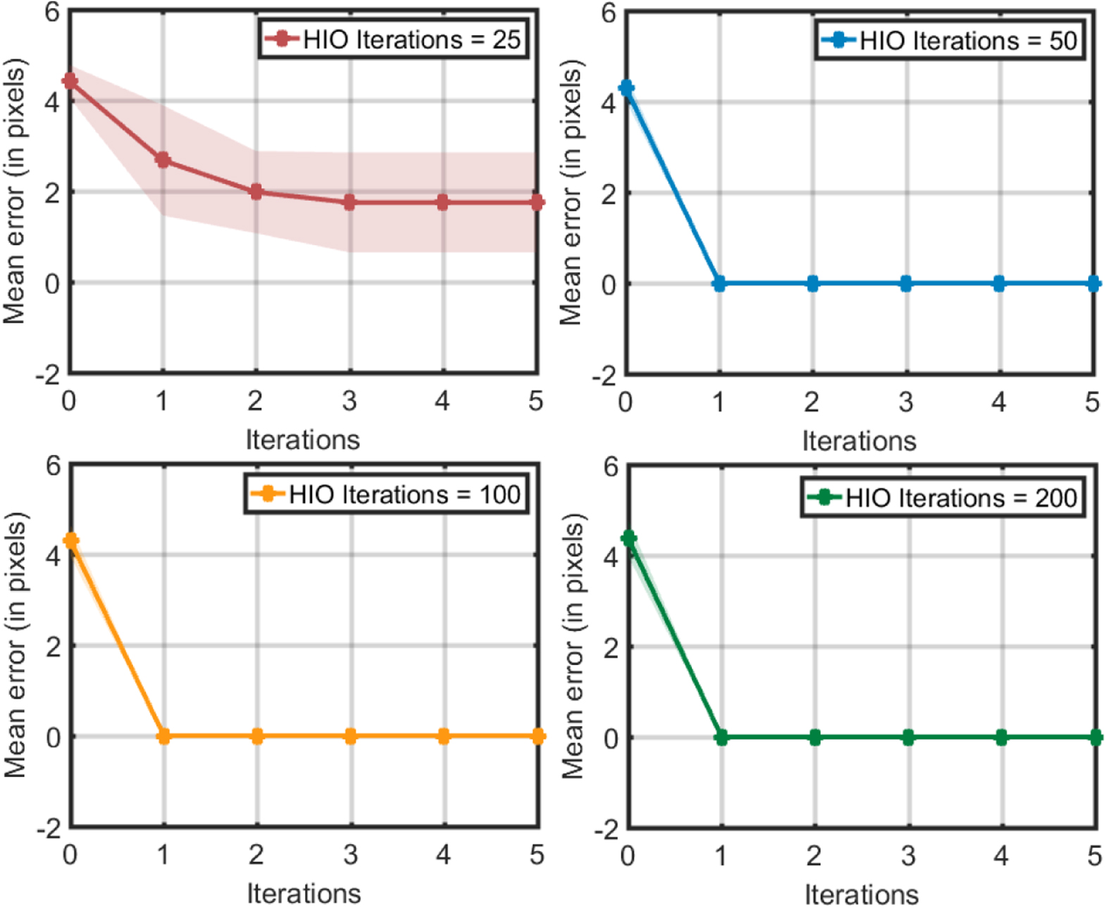
Zoom In Zoom Out Reset image size

On the other hand, as we change the number of HIO iterations while keeping the number of PIE iterations constant, the convergence of the proposed method changes. This can be clearly seen from figures 7 and 8. For each plot, ten simulations were performed where the simulations parameters were same as in section 3.1 except the number of HIO iterations were changing. Figures 7 and 8 show the simulation results for 4 × 4 and 8 × 8 probe positions, respectively. The higher the number of HIO iterations, the better the convergence of the algorithm is. For 50, 100, and 200 iterations of HIO, the probe position errors converge after one iteration of the algorithm. On comparing the results for the case 4 × 4 and 8 × 8, this method is more robust for the 4 × 4 case than for the 8 × 8 case, where the area of the scanned object and the relative overlap were the same. This result may be explained by the fact that the probe is smaller for the 8 × 8 case, leading to a smaller overlapped area. Since this method tries to match the overlapped part of the object to correct the probe positions, the smaller overlapped area influences the results.

Zoom In Zoom Out Reset image size

Zoom In Zoom Out Reset image size

3.3. Simulations in the presence of noise

We also performed the simulations using the intensity patterns corrupted with Poisson noise. The number of photons per diffraction pattern was varied from 10⁶ to 10¹⁰ and the rms probe position errors are shown in figure 9. For each noise level, ten simulations were performed with random initial offsets taken from [−5, 5] pixels for the probe position. Because RAAR is known to outperform HIO in the presence of noise, 100 iterations of RAAR were used instead of HIO. The other parameters for the simulations were the same as mentioned in section 3.1. For the case of 10⁸, 10⁹ and 10¹⁰ photons, most of the time the method gives accurate probe positions. Whereas, for number of photons $\leqslant {10}^{7}$, the method starts to show deviations.

Zoom In Zoom Out Reset image size

3.4. Effect of the initial error and the overlap

To evaluate the performance of the algorithm with varying introduced initial maximum offset in the probe positions and overlap, the simulations results are shown in figure 10. Ten simulations were performed for each overlap and introduced initial maximum offsets in the probe positions. Solid lines show the mean of the final converged probe positions of ten simulations; the semi-transparent patch is the standard deviation of the same. As can be seen from figure 10, all probe positions for all ten simulations converged to the correct probe positions when the initial introduced maximum offset was 5 and 10 pixels. As expected, the algorithm is robust for higher overlap between adjacent probes. For 85% overlap, this method corrected probe positions with 100% accuracy for 15 and 10 pixels of error in these ten simulations.

Zoom In Zoom Out Reset image size

For the comparison in terms of convergence, we have shown the simulation results for the IG method and the proposed method in figure 11. Ten simulations for each method were performed with randomly varying initial probe positions error. The simulation parameters were same as in section 3.1. Figure 11(a) shows the simulation results when the IG method [14] was used to correct the probe positions. For IG method, the first 15 iterations were performed with PIE. Probe position correction started from 16th iteration. From 35th iteration onwards, probe update (ePIE) started. Figure 11(b) shows the simulation results when the proposed method was used to correct the probe positions.

Zoom In Zoom Out Reset image size

The proposed method is correcting probe positions within one iteration. One iteration of the proposed method consists of 10 ePIE, 70 HIO, and 1 cross-correlation. Whereas, for the IG method, the probe positions are corrected within 35 iterations with mean error of 0.80. One iteration of the IG method has 1 ePIE and gradient of intensity (equivalent to two Fourier transforms). The proposed method corrects probe positions with integer pixel accuracy; the IG method corrects with sub-pixel accuracy. A possible suggestion for the proposed method to achieve sub-pixel accuracy is to use matrix multiplication method proposed by Guizar-Sicairos et al [16] as used in CC method to achieve sub-pixel positions correction [11].

In this article, we have proposed an alternative method to correct the probe positions in ptychography which is significantly different from the CC method. The CC method performs cross-correlation between the objects corresponding to consecutive iterations for each probe position. Here, we take the cross-correlation between the objects corresponding to the neighbouring probe positions to match the overlapped region.

In the presence of noise, the proposed method, however, is not as robust as the CC method is. There are a few possible explanations for that. In the presence of noise, some parts of the object have high probability to converge to its twin image or stagnate; thus, they lead to wrong probe positions. Furthermore, since we match the overlapped part of the reconstructed objects corresponding to the neighbouring probe positions, the probe position correction depends on the previous probe position. Therefore, one wrong probe position can propagate this error to the other probe positions as well.

All the simulations presented in this article are based on one assumption: the probe function is zero outside the known area, because the probe function is used as the support constraint while employing HIO. Due to this limitation, it can not be used in every possible application of ptychography. One specific application would be to reconstruct the wavefront, when it is scanned by a mask.

Another important observation is that our method gives better results for a smaller number of probe positions than large number of probe positions, where the scanned area of the object and the relative overlap for the both cases were same. A possible explanation for this is that the size of the probe is smaller for the case of large number of probe positions, which results in an even smaller overlapped area. Since this method tries to match the overlapped region, it does not perform well for a small overlapped area.

We have devised a novel technique which combines HIO and cross-correlation to correct the probe positions in ptychography. This method can correct probe positions with integer pixel accuracy. We have so far not found a case where this method outperforms the IG method or CC method. The results of the study show that it can be used as an alternative method for probe position correction. It has a limitation on the probe function which must be zero outside the defined area of the probe function. Due to this limitation, it can not be used in every possible application of ptychography. We, however, anticipate that this method, for example, can be used for wavefront reconstruction applications. Furthermore, these findings may help us to understand the probe position problem from a different perspective.

The research leading to these results has received funding from the people programme (Marie Curie Actions) of the European Union's Seventh Framework Programme (FP72007-2013) under REA Grant Agreement No. PITN-GA-2013-608082.