
Abstract
Liquid crystals allow for the real-time control of the polarization of light. We describe and provide some experimental examples of the types of general polarization transformations, including universal polarization transformations, that can be accomplished with liquid crystals in tandem with fixed waveplates. Implementing these transformations with an array of liquid crystals, e.g. a spatial light modulator, allows for the manipulation of the polarization across a beam's transverse plane. We outline applications of such general spatial polarization transformations in the generation of exotic types of vector polarized beams, a polarization magnifier, and the correction of polarization aberrations in light fields.
Export citation and abstract BibTeX RIS

Original content from this work may be used under the terms of the Creative Commons Attribution 3.0 licence. Any further distribution of this work must maintain attribution to the author(s) and the title of the work, journal citation and DOI.
1. Introduction
For the last century, polarization manipulation has primarily been conducted using birefringent crystals, known as waveplates, by physically rotating them about a light beam's propagation axis [1–5]. However, waveplates manipulate the polarization uniformly across a beam's transverse profile; that is, they do not allow for spatially varying polarization manipulation. A cell of uniformly aligned liquid crystals acts as a waveplate with a fixed orientation optical axis and a voltage-controlled variable birefringence. When arranged in an array, such as in a liquid-crystal spatial light modulators (LC-SLMs), these devices can spatially tailor the polarization distribution of light by individually controlling the voltage across each cell.
LC-SLMs are widely used for dynamic generation of optical beams possessing particular intensity and phase profiles [6–8]. In the past fifteen years, their inherent birefringence has been used to produce arbitrary spatially polarized beams. However, the schemes to do so are inherently lossy; they rely on spatial and polarization filtering [9–19]. While with classical optics and photonic communications this signal loss is undesirable, in quantum optics it can completely destroy the quantum nature of the light being acted on [20].
In contrast, the polarization transformation schemes that we will present, like the schemes in [21–26], do not require optical loss in order to function. Whereas all of these references focus solely on generating spatially varying polarized states of light, we additionally investigate the implementation of general spatial polarization transformations. Implementing these would enable unprecedented control over spatially varying polarization distributions. Such control could have applications in studying the dynamics and topologies of polarization vortices [27–31], creating exotic polarization topologies in beams, e.g. a Möbius strip in polarization [32], creating novel optical traps for biology and atomic physics [12, 33], for optically guiding and pumping microfluids [34, 35], and for micro-machining [36–38]. In the quantum realm, spatially polarized states can be used to multiply communication bandwidth through superdense coding [39, 40], perform tests of fundamental quantum physics [41, 42], implement quantum key distribution [43–45], and for building measurement devices with quantum-enhanced sensitivities [46, 47].
We limit ourselves to light fields that are perfectly polarized at each spatial point and to transformations that maintain this perfect degree of polarization. Moreover, the transformations should not involve loss, at least in principle. These are known as unitary transformations and are mathematically enacted by Jones Matrices [48]. In turn, these are equivalent to rotations in the Poincaré sphere, as we will review in section 2 and use throughout this paper. In section 3, we will discuss three different kinds of universal unitaries that can be created by combining voltage-controlled liquid crystal cells and fixed waveplates: 1. Variable phase retardation of a fixed but arbitrary polarization. 2. Transformation from an arbitrary polarization state to another arbitrary polarization state. 3. Variable retardation of a variable arbitrary polarization state. At the expense of requiring increasing numbers of waveplates and liquid crystal devices, going from the first to last, these transformations increase in generality. The latter is the most general unitary possible for polarization transformations.
We present an experimental proof-of-concept demonstration of the first kind of transformation outlined above. The experiment is lossy due to technical constraints, but demonstrates that these transformations do not fundamentally require loss to work. The mathematical theory underlying these transformations has not been previously presented. The paper provides explicit formulae and the underlying definitions and conventions that are needed to implement these general polarization transformations in practice. Moreover, the distinct goals of arbitrary polarization generation and arbitrary transformations are often conflated. We clarify the fundamental differences between them and show that they have different requirements and constraints.
2. Background theory
2.1. Waveplates and liquid crystal cells
In this section, we describe the transformation of polarization by birefringent media in terms of rotations on the Poincaré sphere. Since many mutually inconsistent polarization conventions exist in the literature, we give a brief introduction and review of polarization transformations in appendix A, which sets the conventions and notation used in this paper. Light passing through birefringent media, such as a waveplate, gains a phase between the electric field component along the media's optical axis and its orthogonal component. This phase is known as the 'retardance,' Δ. On the Poincaré sphere, the action of a waveplate corresponds to a rotation of an input polarization  by Δ about a rotation axis
  , i.e. one lying in the
 plane at
  from the positive
  axis. Here, Φ is the angle in the laboratory between the fast axis and horizontal,
  , with increasing angle defined to be towards
  . Accordingly, waveplates, such as half-wave plates (
 , HWP) and quarter-wave plates (
 , QWP), can be described by a rotation matrix. More generally, a birefringent waveplate with arbitrary retardance Δ (e.g. an electro-optic modulator or a nematic-phase parallel-aligned liquid crystal) will have the rotation matrix [50],

Since we will be using HWP and QWPs frequently, we define ![${\bf{HWP}}[\![ {\rm{\Phi }}]\!] $](https://content.cld.iop.org/journals/2040-8986/19/9/094003/revision2/joptaa7f65ieqn11.gif)
 and
and ![${\bf{QWP}}[\![ {\rm{\Phi }}]\!] \,\equiv {{\bf{R}}}_{{\bf{k}}(2{\rm{\Phi }},0)}(\pi /2)$](https://content.cld.iop.org/journals/2040-8986/19/9/094003/revision2/joptaa7f65ieqn13.gif) . To avoid any confusion between the reference frames the angles are defined in, an angle expressed in the laboratory frame is written using
. To avoid any confusion between the reference frames the angles are defined in, an angle expressed in the laboratory frame is written using ![$[\![ \cdot ]\!] $](https://content.cld.iop.org/journals/2040-8986/19/9/094003/revision2/joptaa7f65ieqn14.gif) .
.
In the Poincaré sphere, an arbitrary general polarization transformation  consists of a rotation about an arbitrary axis
  by angle ξ (i.e. equation (25)). One can implement this with HWP- and QWPs cascaded in the following sequence:

Ordered first to last, the waveplates the light passes through respectively correspond to the elements in equation (2) from right to left. By an appropriate rotation of each of the three waveplates in the laboratory, any unitary polarization transformation can be created [2]. However, this mechanical rotation will prohibit fast changes of the unitary polarization transformation.
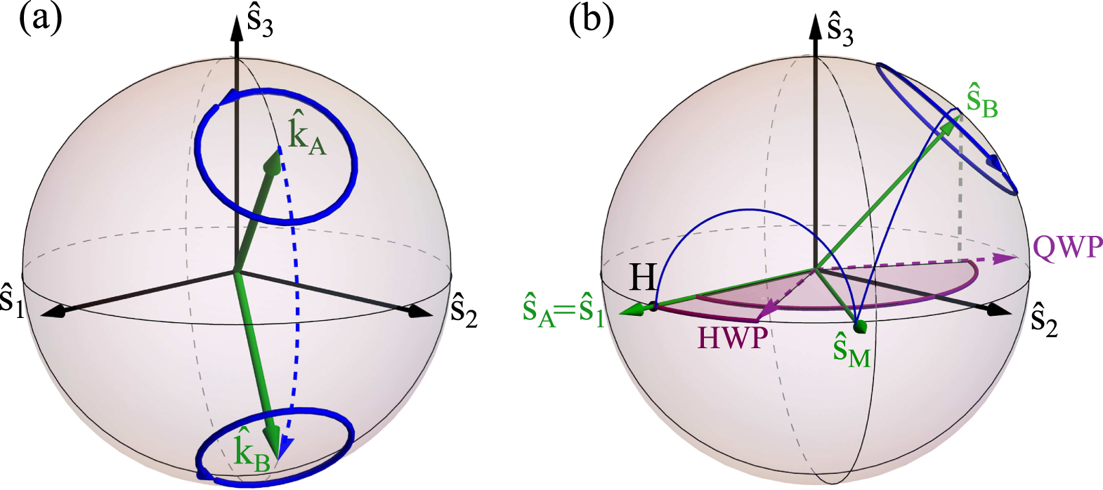
Now suppose we had a birefringent optical element with retardance Δ and rotation axis  , and we wished to convert
  to be
to be  , as in figure 1(a). This could be done by sandwiching the optical element between two sequences of equation (2),

where  is the corresponding rotation matrix of the birefringent optical element, and again, light passes through the elements from right to left. The first sequence of QWP- and HWPs rotates the polarization state
  (positioned at
  on the sphere) to
  (positioned at
  ). The second sequence applies the reverse rotation, rotating it back to
  . In essence, this is a change of basis such that
  , a polarization eigenstate of
  , is unaffected by the waveplates and optical elements—apart from a global phase—and all other polarization states undergo a rotation by Δ about
  .
.

Figure 1. (a) Representation on the Poincaré sphere of the transformation of an arbitrary rotation axis  into another one
  . To perform such a transformation, a sequence of three waveplates (QWP
  HWP
HWP  QWP) converts
  into
into  . (b) For a fixed liquid crystal to perform a rotation about an arbitrary axis
  , one needs to convert the crystal's rotation axis
  to
to  (we take
  ). Consider the passage of state
  through the sequence of waveplates. First a QWP removes the ellipticity of
  , transforming it into
  , which lies on the equator of the sphere. Then, a HWP rotates
  to
to  , the eigenbasis of the liquid crystal. A general polarization state will be rotated by Δ around
  , here. To finish,
  is converted back to
  using the inverse transformation that had converted it from
  to
to  .
.
Download figure:
Standard image High-resolution imageThe most commonly used liquid crystal in optics laboratories is in the nematic phase and is parallel-aligned. It has a variable retardance Δ, but a fixed rotation axis  in the
 plane. Since it has a fixed axis with linear polarization eigenstates, fewer waveplates are necessary in equation (3): only a QWP- and HWP are required to transform any linear polarization to an arbitrary polarization state [1]. The QWP removes the ellipticity from
  rotating it intermediately to
  , a linear polarization state. This state is rotated by the HWP to
  , that is, along the axis of the liquid crystal. Consequently, a four waveplate combination is sufficient for a liquid crystal cell to effectively create an arbitrary rotation
  ,
,

where φ and θ respectively are the azimuthal and polar angles of the target rotation axis  in the Poincaré Sphere (see figure A1(a) for details). The action of the waveplates in equation (4) is shown in figure 1(b) for
  . We will repeatedly use this method of converting rotation axes on the Poincaré sphere in the following sections.
3. General polarization transformations with SLMs
3.1. Spatially variable rotation about a fixed axis
If many liquid crystal cells are arranged in an array, we obtain a spatial light modulator (LC-SLM). Here, For simplicity, we take the fast axis of each liquid crystal cell, and thus the whole LC-SLM, to be along the horizontal. i.e. with  . If one used uniformly H polarized light, a nematic-phase parallel-aligned LC-SLM would function as it is commonly used: as a 'phase-only' spatial light modulator. Here, we consider other input polarizations. The LC-SLM has a rotation matrix equivalent to equation (28) but with a spatially variable retardance (or 'phase distribution') of
  . In this way, LC-SLMs provide the spatial degree of freedom to extend the general polarization transformation in equation (4) to be

The corresponding rotation matrix can then be computed by using equation (1) for the QWP- and HWPs, and equation (28) for the LC-SLM. This configuration gives the possibility for the whole LC-SLM to have an arbitrary fixed rotation axis  , but with a spatially variable rotation angle
  . Figure 1(b) traces the path of a state
  on the Poincaré Sphere as it travels through the waveplates in equation (5).
3.1.1. Practical examples and special cases
Let us look at some practical examples of equation (5).
(i) For a rotation axis on the equator (i.e. 
 plane), the QWPs are not required. In equation (5), the
 ![${\bf{QWP}}[\![ ]\!] $](https://content.cld.iop.org/journals/2040-8986/19/9/094003/revision2/joptaa7f65ieqn65.gif) terms are eliminated and
terms are eliminated and  in the
 ![${\bf{HWP}}[\![ ]\!] $](https://content.cld.iop.org/journals/2040-8986/19/9/094003/revision2/joptaa7f65ieqn67.gif) arguments. For example, for rotations about
arguments. For example, for rotations about  , the diagonal polarization axis, the sequence would be
![$\,=\,{\bf{HWP}}[\![ 112.5^\circ ]\!] $](https://content.cld.iop.org/journals/2040-8986/19/9/094003/revision2/joptaa7f65ieqn70.gif)

![$[\![ 22.5^\circ ]\!] $](https://content.cld.iop.org/journals/2040-8986/19/9/094003/revision2/joptaa7f65ieqn72.gif) .
.
(ii) For rotations about a circular polarization axis, i.e. the  axis, we can remove the HWPs, and use the sequence
![$=\,{\bf{QWP}}[\![ -45^\circ ]\!] $](https://content.cld.iop.org/journals/2040-8986/19/9/094003/revision2/joptaa7f65ieqn75.gif)

![$[\![ 45^\circ ]\!] .$](https://content.cld.iop.org/journals/2040-8986/19/9/094003/revision2/joptaa7f65ieqn77.gif) This sequence has been demonstrated to be particularly useful in creating vector beams such as radial and azimuthal polarization distributions [51]. For this, one begins with uniform horizontally polarized light,
This sequence has been demonstrated to be particularly useful in creating vector beams such as radial and azimuthal polarization distributions [51]. For this, one begins with uniform horizontally polarized light,  . The right-circular component is retarded with respect to the left-circular component resulting in the following polarization distribution after the waveplates and LC-SLM,

The polarization remains linear and is rotated in the laboratory by an angle of  . Thus, the linear polarization direction can vary spatially in an arbitrary manner. However, on the right side of equation (6) there appears an additional phase term that will not explicitly arise in our analysis using rotations in the Poincaré sphere. This phase is addressed in the appendix B.
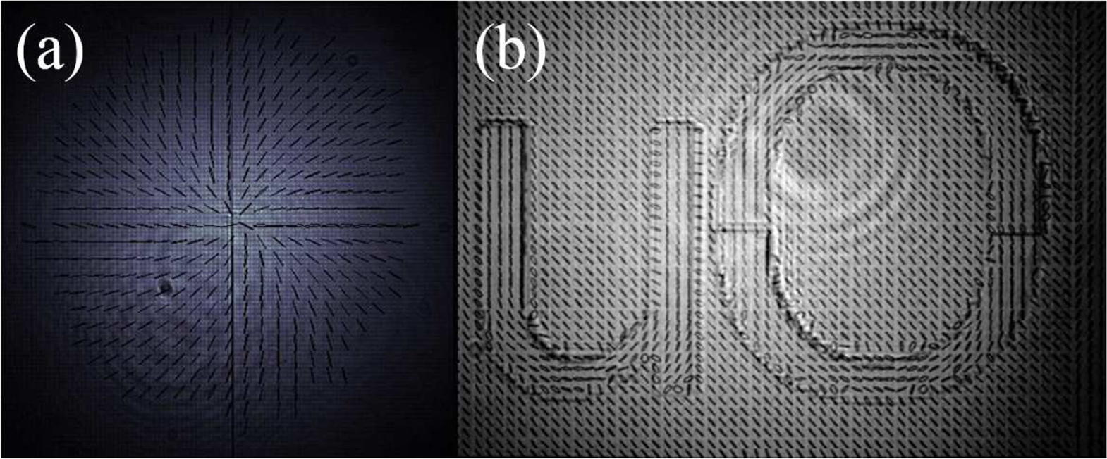
In figure 2(a) we demonstrate that the polarization can be aligned radially. In figure 2(b), the polarization follows the local asymptote of the letters 'uO' (i.e. University of Ottawa). The presence of light at the center may seem surprising since radially polarized beams have a null in intensity at their center, as in a Laguerre–Gauss mode beam. However, in figure 2 we are imaging the LC-SLM surface, at which only the phase, rather than intensity is changed. The resulting field distribution is no longer a 'beam' (for more detail on this subject see appendix B).

Figure 2. Arbitrary linear polarization rotations. (a) Rotations about  axis to produce a radial polarization distribution. The black lines indicate the polarization direction, and the gray-scale gives the intensity. (b) This technique can be used to write arbitrary linear polarization patterns. Here, we write the initials of the University of Ottawa with polarization. See appendix B for experimental details.
Download figure:
Standard image High-resolution image3.2. Transformation from an arbitrary polarization state to another arbitrary polarization state
In our next step in increasing generality, we introduce a scheme to transform an arbitrary input polarization  to another arbitrary output polarization,
  . Both polarization distributions can spatially vary independently. Crucially, though, both
  and
and  must be known at every position
  before implementing the transformation, potentially through prior measurements.
To achieve this transformation, a second LC-SLM is added to the compound device of equation (5), thereby giving the ability to perform rotations about two distinct axes on the Poincaré sphere. Through two rotations about two orthogonal axes, say  and
and  , one can transform any point to any other point on the unit sphere [50]. However, this only holds if one can change the order of the orthogonal rotations. The order will depend on the particular input state and output state. In contrast, we consider a fixed ordering defined by the sequence of LC-SLMs and waveplates in the experimental setup.
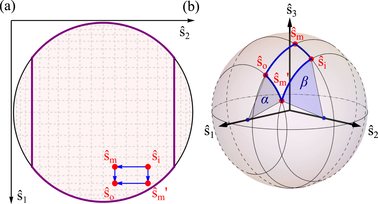
In this section, it is useful to visualize the Poincaré sphere by projecting it on a plane spanned by our two rotation axes,  and
and  . This is shown in figure 3(a). A rotation about
  will take
  to
to  . A following rotation about
  takes
takes  to
to  . Figure 3(b) shows this sequence in a three-dimensional view of the Poincaré sphere for reference. Reversing the order of the rotations would also work, but would instead pass through the intermediate state
  . This will not be generally true though. For many pairs of states
  and
and  , only one ordering will work. In particular, the region outlined in purple in figure 3(a) contains the subset of output states
  that can be reached from the specific
  when rotating about
  first, followed by
  . To understand this, consider moving horizontally in either direction from
  along a line at
  (i.e. a rotation about
  ). In doing so, the largest achievable magnitude for
  is set by the intersection of the line with the circle bounding the Poincaré sphere. That is, at
  .
.

Figure 3. Representation of the transformation of an arbitrary polarization state  into another arbitrary polarization state
  using 2 LC-SLMs. (a) Represents the top view of the Poincaré Sphere depicted in (b). The input state
  can be converted to
  by a succession of one rotation about
  and one rotation about
  . If the order of rotation is not defined, two intermediate points are possible:
  if the state is first rotated about
  , and
, and  if the state is first rotated about
  . However, if the rotation about
  is the first one performed, then, there is only one possibility to go from
  to
to  , which means that it is impossible to reach any polarization state. In this case, the accessible states are in the region outlined in purple.
Download figure:
Standard image High-resolution image3.2.1. Required retardances
Keeping this restriction in mind, we now calculate the required retardances, α and β, of the two LC-SLMs. We assume a configuration which rotates first about  (by α) then
  (by β):

While for brevity we omit an explicit spatial dependence in these vectors and retardances, it should be understood to be implicit in what follows. Specifically, all quantities are for the same transverse point in the light field. In order to transform an input polarization ![${\hat{{\bf{s}}}}_{i}=[{s}_{1}^{i},{s}_{2}^{i},{s}_{3}^{i}]$](https://content.cld.iop.org/journals/2040-8986/19/9/094003/revision2/joptaa7f65ieqn123.gif) to a target output polarization
to a target output polarization ![${\hat{{\bf{s}}}}_{o}=[{s}_{1}^{o},{s}_{2}^{o},{s}_{3}^{o}]$](https://content.cld.iop.org/journals/2040-8986/19/9/094003/revision2/joptaa7f65ieqn124.gif) , one requires the following retardances:
, one requires the following retardances:


where ![${\hat{{\bf{s}}}}_{m}=[{s}_{1}^{m},{s}_{2}^{m},{s}_{3}^{m}]$](https://content.cld.iop.org/journals/2040-8986/19/9/094003/revision2/joptaa7f65ieqn125.gif) is the intermediate point, ·is the dot product, × is the vector cross product,
is the intermediate point, ·is the dot product, × is the vector cross product,  is the vector norm, and
  is the standard signum function with the convention that
  . The function
  is defined as the angle between the positive x axis and the point (x, y), with angle increasing towards the positive y axis. Additionally, we take
  and
and  , in order to ensure that the two LC-SLMs rotate in the positive sense (the angle is increasing).
3.2.2. Applications of arbitrary to arbitrary polarization transformations
We now present three examples of applications that use this transformation.
Ellipticity (de)magnifier: The ellipticity of an input state can be either magnified to be more circular, or demagnified to be more linear. In terms of the Poincaré sphere, changing the ellipticity of state  corresponds to changing the input state's polar angle θ, while maintaining its azimuthal angle φ. This could be used to change a light field containing a spatial polarization distribution with an assortment of elliptical states to one with only linear states. It could also flip the polarization handedness. An example of the rotation paths is shown in figure 4.

Figure 4. Representation of the action of a beam healer/beam ellipticity changer on the Poincaré Sphere. (b) Represents the top view of the Poincaré Sphere depicted in. (a) Here, an elliptical polarization state  , characterized by its coordinates ϕ and θ, can be transformed into any states laying on the great circle passing through the poles and itself using two LC-SLMs. In particular, the state
  can be converted to a linear state, in which case its ellipticity is removed, or converted into the state diametrically opposite on the Poincaré Sphere, in which case the sign of its ellipticity is flipped.
Download figure:
Standard image High-resolution imageBeam healer: Passage through birefringent optical media can undesirably transform a uniform polarization into a non-uniform polarization distribution. This effect could potentially degrade the performance of imaging systems. The method previously introduced in this section (i.e. equation (7)) can restore polarization uniformity.
As discussed in the beginning of the subsection 3.2, when the order of the rotation is fixed, it is only possible to reach a particular subset of output states  (the polarization states included in the purple box in figure 3(a)) from a specific input state
  . However, regardless of the input state
  , it is always possible to reach the poles of the Poincaré Sphere, the right-handed and left-handed circular polarizations. In short, the transformation a beam healer performs on an non-uniform distribution is
  . While transforming an arbitrary polarization to another arbitrary polarization might seem completely general, it is not. We clarify this point in appendix B.
3.3. Spatially variable retardation of a spatially variable polarization
The most general polarization transformation is a rotation by an arbitrary angle ξ about an arbitrary axis  in the Poincaré sphere,
  . This corresponds to a retardation of an arbitrary polarization state. It is a universal unitary transformation for polarization. The axis
  is defined by two free parameters, its spherical coordinates
  , and rotation angle ξ adds a third parameter. It follows that one needs at least three control parameters in order to implement this general transformation. One solution is to use three variable liquid crystals and appropriate fixed waveplates. Considering LC-SLMs, this would implement a different general transformation at each and every transverse position in a light field.
As in section 3.2, the LC-SLMs and waveplates effectively implement rotations about orthogonal axes. The addition of the third LC-SLM, and thus third rotation, allows us to draw upon the concept of proper extrinsic Euler angles, in which a general 3D rotation  can be decomposed into three successive rotations about any two orthogonal axes. Here, we use
  and
and  . Accordingly, we compose the general rotation,

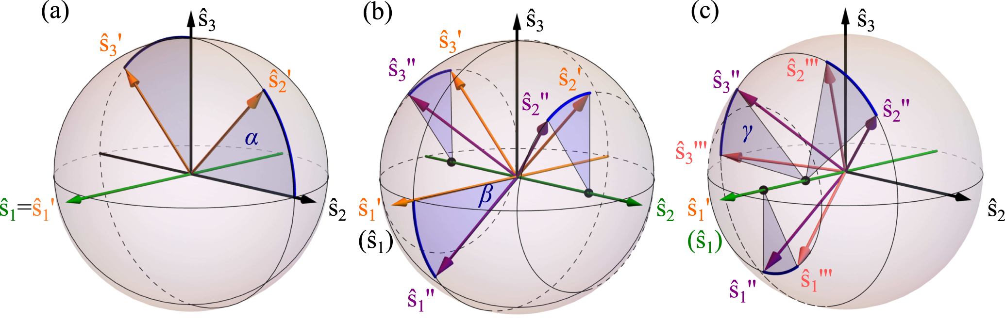
Figure 5 demonstrates the sequential rotations that  performs on the principal axes in terms of the three angles α, β, and γ.

Figure 5. Creation of a general unitary transformation using a sequence of three orthogonal Euler rotations. The first rotation (a) is about  by angle α, the second (b) about
  by β, and the third (c) about
  by γ. From the transformation of the main axes of the Poincaré Sphere (e.g.
  ) one can see that this combination of rotations performs a general 3D rotation (e.g. yaw, pitch, and roll), and, consequently, a general polarization rotation up to a global phase.
Download figure:
Standard image High-resolution image3.3.1. Required retardances
To simplify our notation we write  in the following and define the
  ij matrix element to be the ith row from the top and jth column from the left. In terms of these elements, the angle of each rotation is,


These angles, modded by 2π, are the retardances, 
 and γ, that are applied at each transverse position in the light field by the three LC-SLMs.
These angles are sufficient if one begins with the actual matrix for  , but it may be more useful if they are expressed in terms of the rotation axis
 ![$\hat{{\bf{k}}}=[{k}_{1},\,{k}_{1},\,{k}_{3}]$](https://content.cld.iop.org/journals/2040-8986/19/9/094003/revision2/joptaa7f65ieqn156.gif) and angle ξ,
and angle ξ,


These follow from the matrix expression of the Euler–Rodrigues formula, equation (25) and equations (12)–(14). With these retardances, a completely general polarization unitary can be applied at each transverse position  in a light field.
3.3.2. Applications and examples
Compensation of arbitrary spatially dependent birefringence: Now that we are able to implement a fully universal polarization transformation, we can fully compensate for propagation through optical media. For example, in propagation through a multi-mode optical fiber, stresses and strains in the fiber typically create a small local birefringence that effects supported modes differently. This leads to a spatially dependent unitary  . If one is attempting to use spatial and polarization multiplexing to communicate over such a fiber, this unwanted transformation will cause cross-talk and errors.
Spatially resolved polarization tomography [52] can determine  for the fiber. Once this is known, the apparatus described in this section could be placed after the fiber to implement
  , thereby undoing the transformation. Every spatial mode would emerge with the same polarization that it had at the fiber input.
4. Conclusion
In order to completely control photons and unlock their full potential, scientists must be able to arbitrarily manipulate all four degrees of freedom that fully describe their state: time-frequency, the two transverse position-momentum directions (e.g. x and y), and polarization. In this paper, we described in detail methods to manipulate polarization with liquid crystal devices in conjunction with fixed waveplates. Most generally, we showed how to implement any possible polarization transformation, a universal unitary. Since they are based on liquid crystals, these unitaries can be varied or even completely reconfigured in milliseconds and be computer controlled. Faster operation (e.g. sub-nanosecond) can be achieved by instead using an electro-optic phase modulator [53], which retards light in a similar manner to a liquid crystal.
Combining these methods with SLMs allows for novel and broad control of the spatially varying polarizations of light-fields. Beyond producing vector polarized beams, we proposed a number of applications of these transformations including repairing polarization aberrations in a beam, as a polarization magnifier, and for the compensation of spatial-mode dependent birefringence in fiber-optic communications. Given the broad use of polarization in industrial processes, commercial products, and scientific research, we expect that these general polarization methods will have many more applications in the near future.
Funding
This research was undertaken, in part, thanks to funding from the Canada Research Chairs, NSERC Discovery, Canada Foundation for Innovation, and the Canada Excellence Research Chairs program.
Appendix A.: Polarization conventions and transformations
In this section, we give a brief theoretical review of polarization manipulation. The reader should be aware that there are many conflicting conventions in use for polarization. This section presents a consistent set of definitions (see table A1 for a summary) with which to apply the schemes we introduce in the main text. We characterize the polarization by the manner in which the electric field oscillates. That is, by the normalized complex vector,

where ax and ay are the amplitudes of, and δ the relative phase between, the x and y electric field components, respectively, with  . With
  pointing in the direction of propagation, we use a right-handed co-ordinate system. We follow the convention in [49] by defining right-handed polarization to be clockwise rotating, as seen by the receiver. When
  , where k is an integer, the polarization state is 'elliptical' since the electric field vector traces out an ellipse as a function of time.
Table A1. Table of the conventions used through this paper to define the principal polarization states (i.e. the main axes of the Poincaré sphere), their abbreviations and their representations both in the laboratory frame and on the Poincaré sphere. For the pictorial representation in the Ellipse column, the direction of propagation is towards the observer.
| Laboratory | Poincaré sphere | ||||
|---|---|---|---|---|---|
| Polarization state | Abbrv. | Vector | Ellipse | Stokes vector 
|

|
| Horizontal | H |

|
− |
![$[1,0,0]$](https://content.cld.iop.org/journals/2040-8986/19/9/094003/revision2/joptaa7f65ieqn167.gif)
|

|
| Vertical | V |

|

|
![$[-1,0,0]$](https://content.cld.iop.org/journals/2040-8986/19/9/094003/revision2/joptaa7f65ieqn171.gif)
|

|
| Diagonal | D |

|
/ |
![$[0,1,0]$](https://content.cld.iop.org/journals/2040-8986/19/9/094003/revision2/joptaa7f65ieqn174.gif)
|

|
| Anti-diagonal | A |

|
\ |
![$[0,-1,0]$](https://content.cld.iop.org/journals/2040-8986/19/9/094003/revision2/joptaa7f65ieqn177.gif)
|

|
| Right-hand circular | R |

|

|
![$[0,0,1]$](https://content.cld.iop.org/journals/2040-8986/19/9/094003/revision2/joptaa7f65ieqn181.gif)
|

|
| Left-hand circular | L |

|

|
![$[0,0,-1]$](https://content.cld.iop.org/journals/2040-8986/19/9/094003/revision2/joptaa7f65ieqn185.gif)
|

|
A visually intuitive representation for polarization states is to represent them as points on the surface of a unit sphere, known as the Poincaré sphere [5], as shown in figure A1(a), the polarization equivalent of the Bloch sphere for spin-1/2 or other two-level systems. From the complex vector notation, we can calculate the reduced (normalized) Stokes parameters [5] to obtain a polarization state's position on the sphere,


where φ and θ are the azimuthal and polar angles for the Poincaré sphere. Here, right- and left-handed circular polarizations are respectively mapped to the north and south poles of the sphere. Linear polarization states lie along the equator and elliptical states everywhere else. Orthogonal polarization states are diametrically opposed points. The six polarizations that define the axes are listed in table A1.

Figure A1. The Poincaré sphere and polarization transformations. Polarization states lie on the surface of a sphere that has a radius of one. Horizontal (H) and vertical (V) polarizations define the  axis, diagonal (D) and anti-diagonal (A) states define the
  axis, and right- (R) and left-hand (L) circular define the polar
  axis; each pair lie on the positive and negative ends of the axis, respectively. (a) The polarization state in equation (18) is given by point
 ![$\hat{{\bf{s}}}(\varphi ,\theta )=[{s}_{1},{s}_{2},{s}_{3}]$](https://content.cld.iop.org/journals/2040-8986/19/9/094003/revision2/joptaa7f65ieqn190.gif) on the surface, where si are the Stokes parameters. The polarization state
on the surface, where si are the Stokes parameters. The polarization state  can also be expressed by its coordinates in the spherical system
  . (b) In a polarization transformation, any polarization state is rotated about a fixed axis
  by an angle
  Note: Throughout this paper, the states are represented in red, the axes of rotation in green, the transformation in blue and the definition of angle in purple.
Download figure:
Standard image High-resolution imageIn this paper, we consider only completely polarized states of light. Consequently, the length of the reduced Stokes vector, defined by s0, is identically one, such that all states lie on the surface of the Poincaré sphere. Henceforth, we drop s0 so that a polarization state is described by a three element Stokes vector ![$\hat{{\bf{s}}}={s}_{1}{\hat{{\bf{s}}}}_{1}+{s}_{2}{\hat{{\bf{s}}}}_{2}+{s}_{3}{\hat{{\bf{s}}}}_{3}=[{s}_{1},{s}_{2},{s}_{3}]$](https://content.cld.iop.org/journals/2040-8986/19/9/094003/revision2/joptaa7f65ieqn195.gif) . Alternately, this unit vector can be equivalently expressed in spherical coordinates as
. Alternately, this unit vector can be equivalently expressed in spherical coordinates as  . The angles φ and θ can be related to the complex vector notation via,


In terms of these parameters, we use the conventions listed in table A1.
As shown in figure A1(b), on the Poincaré sphere, polarization transformations—general polarization unitaries—are right-handed rotations of a state  about a unit-length axis
 ![$\hat{{\bf{k}}}=[{k}_{1},{k}_{2},{k}_{2}]=\hat{{\bf{k}}}(\varphi ,\theta )$](https://content.cld.iop.org/journals/2040-8986/19/9/094003/revision2/joptaa7f65ieqn198.gif) by an angle ξ. Mathematically, to perform such a rotation on a Stokes vector, we use a standard three-dimensional active rotation matrix,
by an angle ξ. Mathematically, to perform such a rotation on a Stokes vector, we use a standard three-dimensional active rotation matrix,  . These 3 × 3 matrices are simply the lower-right sub-matrix of the 4 × 4 Mueller rotation matrices used commonly in polarization theory. Using this matrix and writing the Stokes vector as a column, the rotated vector is
  . The general rotation matrix
  is given by a form of the Euler–Rodrigues formula [50],

where  is the 3 × 3 identity matrix, and
  is the cross-product operation matrix of
  ,
,

This gives a rotation matrix of,

The rotation matrices for rotations about the  ,
,  , and
, and  axes can thus be computed from equation (27) using
 ![$\hat{{\bf{k}}}=[1,0,0]$](https://content.cld.iop.org/journals/2040-8986/19/9/094003/revision2/joptaa7f65ieqn208.gif) ,
, ![$[0,1,0]$](https://content.cld.iop.org/journals/2040-8986/19/9/094003/revision2/joptaa7f65ieqn209.gif) , and
, and ![$[0,0,1]$](https://content.cld.iop.org/journals/2040-8986/19/9/094003/revision2/joptaa7f65ieqn210.gif) , respectively,
, respectively,


Appendix B.: Residual spatial phase, relay imaging, and non-universal transformations
In this paper, we concern ourselves only with the the spatial polarization distribution of the beam and neglect spatially varying phases. Nonetheless, the two are linked. There are three physical phases, δ, b, and c, in a single frequency paraxial optical field, 
 . Phase c is an overall global phase that is constant across x and y, and, hence, not relevant for this paper (it is relevant for interference with ancillary fields, as in an interferometer). Phase
  is between fields at different positions. Phase
  is between field polarization components at
  and can vary with x and y. It is this last phase, as well as the magnitude of each polarization component, that we manipulate in this paper.
B.1. Residual phase
However, a residual spatially varying phase  can indeed arise in the polarization transformations that we present. This phase is not evident from rotations in the Poincaré sphere but does arise when using Jones Matrices [48]. If not compensated, this residual phase can have physical consequences. As an example, consider the case where we produce a radially polarized field according to equation (6). On the right-hand side, a residual phase of
  appears. Here,
  , where ϕ is the azimuthal angle about the center of the radial field. It is impact can be understood by considering the left-hand side of equation (6),
  . If an incoming optical field had a Gaussian transverse profile, the left-handed component
  would be unchanged, whereas the right-handed component
  would receive an azimuthally varying phase carrying
  units of orbital angular momentum. This phase profile causes the right-handed light-field to no longer be a solution to the paraxial wave equation. Hence, it is no longer a 'beam' in the sense that it does not maintain its spatial and polarization distribution upon propagation (up to a scale factor). We experimentally demonstrated this by allowing the radial field in figure B1(a) to propagate 10 cm further. The polarization and intensity distribution at this point is shown in figure B1(b). We call this the 'far-field'. Physically, the residual phase arises from a variety of causes including, but not limited to, the Pancharatnam–Berry phase. The latter is known to affect propagation, as was in demonstrated in [54].

Figure B1. Rotations about  axis to produce radial polarization distribution. We can see the pictures of the beam and its polarization state at various positions in the imaging plane (a) and 'far-field' (b).
Download figure:
Standard image High-resolution imageIn all three types of transformations, a single extra SLM is all that is required to correct this residual phase  . Our methods control the phase
  between
  and
and  polarizations at any particular point. Therefore, if we phase-shift
  by
by  with a single extra SLM, we would have
  . Setting
  would cancel the residual phase. One would then also need to pre-compensate in our initial transformation by increasing
  by
by  . Formulas for
  can be found using the Jones matrix formalism.
B.2. Imaging requirements for general polarization manipulation
Figure B1 shows there are notable differences between the output polarization distribution at the image plane of the LC-SLM (near-field) and after propagation (far-field) for the same input polarization and LC-SLM phase pattern,  . However, throughout this paper we assumed that LC-SLMs can be placed in series while acting on the same unchanged optical field. To achieve this, the field at one LC-SLM is imaged onto the next with a 4-f system. The latter acts as a relay imaging system with a one-to-one magnification ratio.
Ideally, in order to create a simple setup with high transmissivity, the LC-SLMs would be transmissive and placed in a line. However, reflective LC-SLMs often have better performance specifications. A reflective setup usually involves picking off a beam that is reflected at a small angle. Since, the pick-off mirror acts as an aperture this can dramatically change the optical field imaged by a 4-f setup. Our setup, shown in figure B2, uses a reflective LC-SLM. In order to separate the reflected beam from incident beam we use a non-polarizing beam-splitter (NPBS) instead of a pick-off mirror. The drawback is that this NPBS introduces loss. Nonetheless, the setup allows us to test the transformations, which are lossless in principle.

Figure B2. Experimental setup to perform a rotation about  . A diode laser (635 nm) is prepared to be left-handed circular with a quarter-wave plate (QWP), and then reflected off of an LC-SLM (LCOS-SLM X10468, Hamamatsu, Japan), which imprints the desired spatially varying phase (i.e. rotation angle or 'retardance'). A non-polarizing beam-splitter (NPBS) splits off half of the light to be analyzed. A second quarter-wave plate converts circular states back to linear states. A 4-f imaging system is used to image the plane of the LC-SLM onto a CCD camera. We use short focal length (f = 100 mm, diameter = 25.4 mm) doublet lenses in order to have a high numerical aperture. The polarization of the light is then determined pixel by pixel via polarization tomography (i.e. Stokes polarimetry) with a half-wave plate (HWP), quater-wave plate, and polarizing beam-splitter (PBS) [55].
Download figure:
Standard image High-resolution image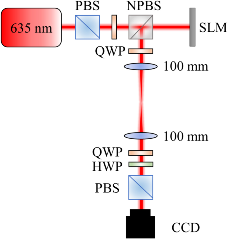
B.3. Arbitrary to arbitrary polarization versus universal transformations
While transforming an arbitrary polarization to another arbitrary polarization might seem completely general, it is not. The most general rotation is  , whereas the transformation that is implemented through this method is
  . The latter implements
  , which takes
  . It also links the polarization states diametrically opposed to these on the Poincaré sphere,
  . However,
  does not fix the retardance ζ between
  and
and  . This retardance is crucial when considering how
  transforms any input state other than
  . Polarizations that are a superposition of
  and
and  will transform in an undetermined way.