Topological charge conservation in stochastic optical fields

Optical speckle, which is produced when light scatters from a rough surface, have been studied extensively [1, 2]. Such optical speckle fields contain distributions of phase singularities, popularly called optical vortices [3], at the complex zeros of the optical field. These phase singularities carry topological charges¹ of either +1 or −1, depending on the handedness of the surrounding phase wrapping. Studies of the statistical properties of optical vortices in such speckle optical fields [4–14] revealed that the vortices are evenly distributed, have a density given by the second derivative of the optical field's autocorrelation function at the origin [4], and that neighbouring vortices tend to have opposite topological charges [9]. The latter implies that the topological charge densities of speckle fields are on average zero [12, 14].

Stochastic optical fields are close relatives of speckle fields. They are a little less random than speckle fields, in that they can contain additional transverse correlations. These correlations have a number of interesting consequences, one of which is the fact that such stochastic optical fields can have nonzero topological charge densities [15], but such topological charge distributions would integrate to a zero net topological charge for the total optical field and they would eventually decay to zero during propagation. Nevertheless, the existence of nontrivial topological charge densities opens up a new avenue for investigations into the nature of stochastic light. Here, we will assume that the stochastic optical fields are monochromatic, paraxial, normally distributed and that one can ignore polarization.

When viewed in three-dimensions, the complex zeros of optical fields form lines. The topological charges of these zeros define a topological charge flow along these lines, such that for positive (negative) topological charges the flow is in (opposite to) the direction of propagation.

Topological charge is locally conserved: the total topological charge flowing into, or out of, a closed surface is zero. This fact implies the existence of a topological charge current in stochastic optical fields. One should be able to express this topological charge current in terms of the local correlation functions of the stochastic optical field and its transverse derivatives. The component of this current in the direction of propagation is the topological charge density. While the expression for the topological charge density is known [16], the nature of the transverse part of the current is not.

Here, we derive the complete conserved current for the topological charge in stochastic optical fields. In other words, we obtain the expression for the transverse part of the topological charge current in terms of the local correlation functions of the stochastic optical field, which, together with the topological charge density, forms the full three-dimensional topological charge current. Two approaches are used to obtain the expression for the transverse part of the current. We demonstrate that the expression for the complete current obeys a conservation equation. The expression for the topological charge current is used to investigate the evolution of the topological charge flow in a stochastic optical field with a one-dimensional initial topological charge density.

2.1. Notation

The quantities of interest are here expressed in terms of local two-point correlation functions, such as, for example, the intensity $I({\bf{x}})=\langle {g}_{}^{}{\bar{g}}_{}\rangle$, where g represents the complex optical field, $\bar{g}$ represents its complex conjugate and $\langle \cdot \rangle$ denotes the ensemble average. The local two-point correlation functions can also involve derivatives of the optical field. As a result, one has an endless set of possible local two-point correlation functions

$$\begin{eqnarray}&&\{\langle {g}_{}^{}{\bar{g}}_{}\rangle ,\langle {g}_{x}^{}{\bar{g}}_{}\rangle ,\langle {g}_{y}^{}{\bar{g}}_{x}\rangle ,\langle {g}_{}^{}{\bar{g}}_{{xx}}\rangle ,\langle {g}_{y}^{}{\bar{g}}_{{xy}}\rangle ,...\},\end{eqnarray} \tag{ 1 }$$

where the subscripts indicate transverse derivatives with respect to x and y. The propagation direction is chosen to be the z-direction.

The quantities that we are interested in, usually contain polynomials of local correlation functions. These polynomials are invariant under transverse coordinate rotations [16]. As a result, the polynomials in these quantities are singlets under the SO(2) Lie group that represents the coordinate rotations on the transverse plane. All such singlets that are composed of local two-point correlation functions, involving the optical field and/or its derivatives, can be represented in terms of a finite set of irreducible singlets, which cannot be simplified further.

A complete discussion of these singlets is beyond the scope of the current paper. We will only need a few of them. Scalar singlets that only involve the optical field and first derivatives of the optical field are denoted by τ's. There are only 14 such irreducible singlets $\{{\tau }_{0}...{\tau }_{13}\}$, which includes the intensity ${\tau }_{0}$. They are listed in the appendix in [16]. When the scalar singlets also include second or higher derivatives of the optical field, we denote them by ψ's. There are also vectorial singlets. When such vectorial singlets only involve the optical field and first derivatives of the optical field we denote them by ${\boldsymbol{v}}$'s and when they also include second or higher derivatives, we simply denote them by ${\bf{V}}$'s. Here, we will provide the expressions for these irreducible singlets as they occur. The irreducible singlets are often related to each other via differential operations. Sometimes they also have some physical interpretation. We will provide some of these relationships and mention their physical interpretations where possible.

2.2. Phase gradient

A quantity that plays a central role in the discussion is the expectation value of the phase gradient. One can define the phase of a complex optical field by

$$\begin{eqnarray}&&\theta ({\bf{x}})=\displaystyle \frac{-{\rm{i}}}{2}\mathrm{ln}\left[\displaystyle \frac{g({\bf{x}})}{\bar{g}({\bf{x}})}\right].\end{eqnarray} \tag{ 2 }$$

The gradient then becomes

$$\begin{eqnarray}&&{\rm{\nabla }}\theta ({\bf{x}})=\displaystyle \frac{{\rm{i}}[g({\bf{x}}){\rm{\nabla }}\bar{g}({\bf{x}})-\bar{g}({\bf{x}}){\rm{\nabla }}g({\bf{x}})]}{2\;g({\bf{x}})\bar{g}({\bf{x}})}.\end{eqnarray} \tag{ 3 }$$

Computing the expectation value of the transverse phase gradient, one finds²

$$\begin{eqnarray}&&\langle {{\rm{\nabla }}}_{\perp }\theta \rangle ={{\bf{F}}}_{\perp }=\displaystyle \frac{{{\boldsymbol{v}}}_{2}}{2{\tau }_{0}},\end{eqnarray} \tag{ 4 }$$

where the subscript ⊥ denotes the transverse part of a quantity, ${\tau }_{0}=\langle {g}_{}^{}{\bar{g}}_{}\rangle$ and

$$\begin{eqnarray}&&{{\boldsymbol{v}}}_{2}=-{\rm{i}}[(\langle {g}_{x}^{}{\bar{g}}_{}\rangle -\langle {g}_{}^{}{\bar{g}}_{x}\rangle )\hat{x}+(\langle {g}_{y}^{}{\bar{g}}_{}\rangle -\langle {g}_{}^{}{\bar{g}}_{y}\rangle )\hat{y}],\end{eqnarray} \tag{ 5 }$$

is an irreducible vectorial singlet.

The expectation value of the full three-dimensional phase gradient is³

$$\begin{eqnarray}&&\langle {\rm{\nabla }}\theta \rangle ={\bf{F}}=\displaystyle \frac{{{\boldsymbol{v}}}_{2}}{2{\tau }_{0}}-\displaystyle \frac{{\psi }_{1}}{4k{\tau }_{0}}\hat{z}-k\hat{z},\end{eqnarray} \tag{ 6 }$$

where k is the wavenumber and

$$\begin{eqnarray}&&{\psi }_{1}=\langle {g}_{{xx}}^{}{\bar{g}}_{}\rangle +\langle {g}_{}^{}{\bar{g}}_{{xx}}\rangle +\langle {g}_{{yy}}^{}{\bar{g}}_{}\rangle +\langle {g}_{}^{}{\bar{g}}_{{yy}}\rangle ={\rm{\nabla }}\cdot {{\boldsymbol{v}}}_{1}-2{\tau }_{1},\end{eqnarray} \tag{ 7 }$$

is a singlet involving second derivatives of the optical field. In equation (7), we also express the singlet in terms of the divergence of

$$\begin{eqnarray}&&{{\boldsymbol{v}}}_{1}={\rm{\nabla }}{\tau }_{0}=(\langle {g}_{x}^{}{\bar{g}}_{}\rangle +\langle {g}_{}^{}{\bar{g}}_{x}\rangle )\hat{x}+(\langle {g}_{y}^{}{\bar{g}}_{}\rangle +\langle {g}_{}^{}{\bar{g}}_{y}\rangle )\hat{y}\end{eqnarray} \tag{ 8 }$$

(the gradient of the intensity) and

$$\begin{eqnarray}&&{\tau }_{1}=\langle {g}_{x}^{}{\bar{g}}_{x}\rangle +\langle {g}_{y}^{}{\bar{g}}_{y}\rangle ,\end{eqnarray} \tag{ 9 }$$

associated with the magnitude squared of the gradient of the optical field.

2.3. Topological charge density

For scalar stochastic optical fields that are monochromatic, paraxial and normally distributed, one can compute the topological charge density to obtain [16]

$$\begin{eqnarray}&&T=\displaystyle \frac{{\tau }_{0}{\tau }_{2}-{\tau }_{6}}{2\pi {\tau }_{0}^{2}},\end{eqnarray} \tag{ 10 }$$

where

$$\begin{eqnarray}&&{\tau }_{2}={\rm{i}}(\langle {g}_{x}^{}{\bar{g}}_{y}\rangle -\langle {g}_{y}^{}{\bar{g}}_{x}\rangle ),\end{eqnarray} \tag{ 11 }$$

$$\begin{eqnarray}&&{\tau }_{6}={\rm{i}}(\langle {g}_{x}^{}{\bar{g}}_{}\rangle \langle {g}_{}^{}{\bar{g}}_{y}\rangle -\langle {g}_{}^{}{\bar{g}}_{x}\rangle \langle {g}_{y}^{}{\bar{g}}_{}\rangle ).\end{eqnarray} \tag{ 12 }$$

The singlet ${\tau }_{2}$ is proportional to the local orbital angular momentum density of the stochastic optical field and ${\tau }_{6}$ is proportional to the cross-product between the gradient of the phase and the gradient of the intensity ${{\boldsymbol{v}}}_{1}\times {{\boldsymbol{v}}}_{2}=2{\tau }_{6}$.

The transverse curl of the transverse phase gradient, which is given in equation (4), is proportional to the topological charge density [16]:

$$\begin{eqnarray}&&{{\rm{\nabla }}}_{\perp }\times {{\bf{F}}}_{\perp }=2\pi \ T\hat{z}.\end{eqnarray} \tag{ 13 }$$

This is a result of the fact that derivatives do not commute for phase functions [17]. The commutator of the transverse derivatives applied to the phase function gives the distribution of phase singularities, which is equal to $2\pi$ times the topological charge density:

$$\begin{eqnarray}&&[{\partial }_{x},{\partial }_{y}]\theta (x,y)=2\pi \ T.\end{eqnarray} \tag{ 14 }$$

The fact that the topological charge is conserved can be expressed as a conservation equation, given by

$$\begin{eqnarray}&&2\pi \ {\partial }_{z}T+{{\rm{\nabla }}}_{\perp }\cdot {{\bf{J}}}_{{\rm{T}}}=0.\end{eqnarray} \tag{ 15 }$$

The transverse topological charge current ${{\bf{J}}}_{{\rm{T}}}$ has thus far been unknown. Next, we will derive this transverse topological charge current using two different approaches.

3.1. Three-dimensional curl of the phase gradient

The first approach is to compute the curl of the full three-dimensional phase gradient given in equation (6). One can view the full three-dimensional topological charge current as the combination of the three topological charge densities that are obtained on the (x–y), (x–z) and (y–z) planes, respectively. For each of these three the topological charge density would be given by the two-dimensional curl restricted to that plane, in the same way that T is produced in equation (13). By combining these three two-dimensional curl operations into one three-dimensional curl operation, one obtains the three-dimensional topological charge current, given below. The resulting vector field ${{\bf{J}}}_{{\rm{full}}}={\rm{\nabla }}\times {\bf{F}}$ would be a conserved current for the topological charge, because ${\rm{\nabla }}\cdot ({\rm{\nabla }}\times {\bf{F}})=0$.

Computing the curl of equation (6), one finds

$$\begin{eqnarray}&&{\rm{\nabla }}\times {\bf{F}}=2\pi \ T\hat{z}+\hat{z}\times {{\bf{V}}}_{{\rm{T}}},\end{eqnarray} \tag{ 16 }$$

where

$$\begin{eqnarray}&&{{\bf{V}}}_{{\rm{T}}}=\displaystyle \frac{{\partial }_{z}{{\boldsymbol{v}}}_{2}}{2{\tau }_{0}}-\displaystyle \frac{{{\boldsymbol{v}}}_{2}{\partial }_{z}{\tau }_{0}}{2{\tau }_{0}^{2}}+\displaystyle \frac{{{\rm{\nabla }}}_{\perp }{\psi }_{1}}{4k{\tau }_{0}}-\displaystyle \frac{{\psi }_{1}{{\rm{\nabla }}}_{\perp }{\tau }_{0}}{4k{\tau }_{0}^{2}}.\end{eqnarray} \tag{ 17 }$$

The full three-dimensional curl involves z-derivatives, which are converted to second-order transverse derivatives with the aid of the paraxial wave equation

$$\begin{eqnarray}&&{\partial }_{z}\langle {g}_{p}^{}{\bar{g}}_{q}\rangle =\displaystyle \frac{-{\rm{i}}}{2k}(\langle {g}_{{xxp}}^{}{\bar{g}}_{q}\rangle -\langle {g}_{p}^{}{\bar{g}}_{{xxq}}\rangle +\langle {g}_{{pyy}}^{}{\bar{g}}_{q}\rangle -\langle {g}_{p}^{}{\bar{g}}_{{qyy}}\rangle ),\end{eqnarray} \tag{ 18 }$$

where p and q denote combinations of x's and y's. As a result, we obtain an expression that only involves transverse derivatives, even though we applied a three-dimensional differential operator. The reason why we want to express the quantities only in transverse derivatives is because one usually observes the optical field in a transverse plane, which implies that one only has access to the transverse derivatives of the optical field.

The following differential relationships exist among the irreducible singlets

$$\begin{eqnarray}&&{{\rm{\nabla }}}_{\perp }{\tau }_{0}={{\boldsymbol{v}}}_{1},\end{eqnarray} \tag{ 19 }$$

$$\begin{eqnarray}&&{\partial }_{z}{\tau }_{0}=-\displaystyle \frac{{\psi }_{2}}{2k},\end{eqnarray} \tag{ 20 }$$

$$\begin{eqnarray}&&{{\rm{\nabla }}}_{\perp }{\psi }_{1}={{\bf{V}}}_{3}+{{\bf{V}}}_{4},\end{eqnarray} \tag{ 21 }$$

$$\begin{eqnarray}&&{\partial }_{z}{{\boldsymbol{v}}}_{2}=\displaystyle \frac{{{\bf{V}}}_{3}-{{\bf{V}}}_{4}}{2k},\end{eqnarray} \tag{ 22 }$$

where

$$\begin{eqnarray}{{\bf{V}}}_{3} & = & (\langle {g}_{{xx}}^{}{\bar{g}}_{x}\rangle +\langle {g}_{x}^{}{\bar{g}}_{{xx}}\rangle +\langle {g}_{x}^{}{\bar{g}}_{{yy}}\rangle +\langle {g}_{{yy}}^{}{\bar{g}}_{x}\rangle )\hat{x}\\ & & +(\langle {g}_{{xx}}^{}{\bar{g}}_{y}\rangle +\langle {g}_{y}^{}{\bar{g}}_{{xx}}\rangle +\langle {g}_{{yy}}^{}{\bar{g}}_{y}\rangle +\langle {g}_{y}^{}{\bar{g}}_{{yy}}\rangle )\hat{y},\end{eqnarray} \tag{ 23 }$$

$$\begin{eqnarray}{{\bf{V}}}_{4} & = & (\langle {g}_{{xx}}^{}{\bar{g}}_{x}\rangle +\langle {g}_{x}^{}{\bar{g}}_{{xx}}\rangle +\langle {g}_{x}^{}{\bar{g}}_{{yy}}\rangle +\langle {g}_{{yy}}^{}{\bar{g}}_{x}\rangle )\hat{x}\\ & & +(\langle {g}_{{xx}}^{}{\bar{g}}_{y}\rangle +\langle {g}_{y}^{}{\bar{g}}_{{xx}}\rangle +\langle {g}_{{yy}}^{}{\bar{g}}_{y}\rangle +\langle {g}_{y}^{}{\bar{g}}_{{yy}}\rangle )\hat{y}\end{eqnarray} \tag{ 24 }$$

and

$$\begin{eqnarray}&&{\psi }_{2}={\rm{i}}(\langle {g}_{{xx}}^{}{\bar{g}}_{}\rangle -\langle {g}_{}^{}{\bar{g}}_{{xx}}\rangle +\langle {g}_{{yy}}^{}{\bar{g}}_{}\rangle -\langle {g}_{}^{}{\bar{g}}_{{yy}}\rangle ).\end{eqnarray} \tag{ 25 }$$

Substituting equations (19) to (22) into equation (17), we obtain the following expression for ${{\bf{V}}}_{{\rm{T}}}$

$$\begin{eqnarray}&&{{\bf{V}}}_{{\rm{T}}}=\displaystyle \frac{{{\boldsymbol{v}}}_{2}{\psi }_{2}-{{\boldsymbol{v}}}_{1}{\psi }_{1}}{4k{\tau }_{0}^{2}}+\displaystyle \frac{{{\bf{V}}}_{3}}{2k{\tau }_{0}}.\end{eqnarray} \tag{ 26 }$$

The transverse current is therefore given by

$$\begin{eqnarray}&&{{\bf{J}}}_{{\rm{T}}}^{(a)}=\displaystyle \frac{(\hat{z}\times {{\boldsymbol{v}}}_{2}){\psi }_{2}-(\hat{z}\times {{\boldsymbol{v}}}_{1}){\psi }_{1}}{4k{\tau }_{0}^{2}}+\displaystyle \frac{(\hat{z}\times {{\bf{V}}}_{3})}{2k{\tau }_{0}}.\end{eqnarray} \tag{ 27 }$$

3.2. Changing the order of differentiation

The second approach is to apply a z-differentiation to equation (13) and then change the order of differentiation

$$\begin{eqnarray}&&{\partial }_{z}({{\rm{\nabla }}}_{\perp }\times {{\bf{F}}}_{\perp })={{\rm{\nabla }}}_{\perp }\times ({\partial }_{z}{{\bf{F}}}_{\perp }).\end{eqnarray} \tag{ 28 }$$

In two-dimensions, one can convert a curl operation into a divergence

$$\begin{eqnarray}&&{{\rm{\nabla }}}_{\perp }\times {\bf{V}}={{\rm{\nabla }}}_{\perp }\cdot ({\bf{V}}\times \hat{z})\hat{z}.\end{eqnarray} \tag{ 29 }$$

Applying equation (29) to equation (28), one obtains

$$\begin{eqnarray}&&{\partial }_{z}({{\rm{\nabla }}}_{\perp }\times {{\bf{F}}}_{\perp })+{{\rm{\nabla }}}_{\perp }\cdot (\hat{z}\times {\partial }_{z}{{\bf{F}}}_{\perp })=0.\end{eqnarray} \tag{ 30 }$$

The z-derivative of the transverse phase gradient is

$$\begin{eqnarray}&&{\partial }_{z}{{\bf{F}}}_{\perp }=\displaystyle \frac{{\partial }_{z}{{\boldsymbol{v}}}_{2}}{2{\tau }_{0}}-\displaystyle \frac{{{\boldsymbol{v}}}_{2}{\partial }_{z}{\tau }_{0}}{2{\tau }_{0}^{2}}=\displaystyle \frac{{{\bf{V}}}_{3}-{{\bf{V}}}_{4}}{4k{\tau }_{0}}+\displaystyle \frac{({{\boldsymbol{v}}}_{2}){\psi }_{2}}{4k{\tau }_{0}^{2}},\end{eqnarray} \tag{ 31 }$$

where we used equations (20) and (22). As a result, we get the conservation equation

$$\begin{eqnarray}&&2\pi \ {\partial }_{z}T+{{\rm{\nabla }}}_{\perp }\cdot {{\bf{J}}}_{{\rm{T}}}^{(b)}=0,\end{eqnarray} \tag{ 32 }$$

where, in this case, the transverse current is

$$\begin{eqnarray}&&{{\bf{J}}}_{{\rm{T}}}^{(b)}=\displaystyle \frac{(\hat{z}\times {{\boldsymbol{v}}}_{2}){\psi }_{2}}{4k{\tau }_{0}^{2}}+\displaystyle \frac{(\hat{z}\times {{\bf{V}}}_{3})-(\hat{z}\times {{\bf{V}}}_{4})}{4k{\tau }_{0}}.\end{eqnarray} \tag{ 33 }$$

The expressions of the transverse currents obtained in equations (27) and (33), are different. This is because such conserved currents are only unique up to the addition of a divergence-free vector field. In this case, the difference is

$$\begin{eqnarray}&&{\rm{\Delta }}{{\bf{J}}}_{{\rm{T}}}={{\bf{J}}}_{{\rm{T}}}^{(a)}-{{\bf{J}}}_{{\rm{T}}}^{(b)}=\displaystyle \frac{(\hat{z}\times {{\bf{V}}}_{3})+(\hat{z}\times {{\bf{V}}}_{4})}{4k{\tau }_{0}}-\displaystyle \frac{(\hat{z}\times {{\boldsymbol{v}}}_{1}){\psi }_{1}}{4k{\tau }_{0}^{2}},\end{eqnarray} \tag{ 34 }$$

which is the divergence of the cross-product of $\hat{z}$ and the gradient of the z-component of the full three-dimensional phase gradient given in equation (6).

3.3. Full three-dimensional topological charge current

Although equation (33) gives a valid expression for the transverse part of a conserved current, it does not have the same physical justification to identify it as the transverse part of the topological charge current. Therefore, we prefer the expression in equation (27) as the transverse part of the topological charge current.

The full three-dimensional topological charge current is therefore given by

$$\begin{eqnarray}&&{{\bf{J}}}_{{\rm{full}}}=\displaystyle \frac{(\hat{z}\times {{\boldsymbol{v}}}_{2}){\psi }_{2}-(\hat{z}\times {{\boldsymbol{v}}}_{1}){\psi }_{1}}{4k{\tau }_{0}^{2}}+\displaystyle \frac{(\hat{z}\times {{\bf{V}}}_{3})}{2k{\tau }_{0}}+2\pi T\hat{z},\end{eqnarray} \tag{ 35 }$$

where ${\boldsymbol{v}}$₁, ${\boldsymbol{v}}$₂, ${\psi }_{1}$, ${\psi }_{2}$, ${{\bf{V}}}_{3}$ and T are defined in equations (5), (7), (8), (10), (23) and (25) respectively.

With the aid of equations (16) and (29), one can express the conservation equation in a different way

$$\begin{eqnarray}&&2\pi \ {\partial }_{z}T+{{\rm{\nabla }}}_{\perp }\times {{\bf{V}}}_{{\rm{T}}}=0,\end{eqnarray} \tag{ 36 }$$

where ${{\bf{V}}}_{{\rm{T}}}$ is defined in equation (17).

To demonstrate the application of the conserved topological charge current, we considered both a one-dimensional topological charge density and a two-dimensional topological charge density. In both cases the topological charge current is found to be conserved by obeying equation (36). Due to the extreme complexity of the expressions for the two-dimensional case (similar to the case previously considered in [18]), we only discuss the one-dimensional case here.

The one-dimensional topological charge distribution, which is the same case that has been considered in [15], is produced with the aid of the interferometric setup shown in figure 1 (figure 2 of [15]). An input laser beam is divided by a 50/50 beam splitter, resulting in two beams. They are passed through ground glass plates to produce two mutually uncorrelated speckle fields. Two Mach–Zehnder interferometers are embedded in the respective beams to produce sinusoidal interference patterns in the respective speckle fields. These speckle fields are then combined in such a way that the dark bands of one interference pattern overlaps with the bright bands of the other. At the same time, the beams have a relative tilt along the homogeneous direction. One thus obtains a combined speckle field with a constant average intensity and a one-dimensional sinusoidal topological charge density.

Zoom In Zoom Out Reset image size

The far-field pattern (angular spectrum) of the optical field that is produced by the setup in figure 1, is shown diagrammatically in figure 2 (figure 3 of [15]). Each disc represents the angular spectrum of a (random) speckle field. Discs with the same color are shifted versions of the same spectrum and those with different colors are different, mutually uncorrelated fields. The enclosed numbers are the relative phases of the beams in the superposition. To ensure that the scale over which the topological charge density varies is much larger than the average separation distance between phase singularities, the size of the beams on the Fourier plane W₀ must be much larger than the separation distance between the beams, contrary to the way it is shown in figure 2.

Zoom In Zoom Out Reset image size

The optical field that is produced by the setup in figure 1 can be expressed as

$$\begin{eqnarray}g({\bf{x}}) & = & \displaystyle \int G(a,b)\mathrm{exp}[-{\rm{i}}2\pi ({ax}+{by})\\ & & +{\rm{i}}\pi ({a}^{2}+{b}^{2})\lambda z]{\rm{d}}a{\rm{d}}b,\end{eqnarray} \tag{ 37 }$$

where we include the paraxial propagation kernel to produce a z-dependence, with λ being the wavelength, and where $G(a,b)$ is the angular spectrum given as the superposition of four random fields

$$\begin{eqnarray}G(a,b) & = & {G}_{1}(a+{a}_{0},b-{b}_{0})+{G}_{1}(a-{a}_{0},b-{b}_{0})\\ & & +{\rm{i}}{G}_{2}(a+{a}_{0},b+{b}_{0})\\ & & -{\rm{i}}{G}_{2}(a-{a}_{0},b+{b}_{0}),\end{eqnarray} \tag{ 38 }$$

with a₀ and b₀ being the x- and y-offsets on the Fourier plane, as shown in figure 2. The two uncorrelated spectra are modeled by

$$\begin{eqnarray}&&{G}_{s}(a,b)={\chi }_{s}(a,b)h(a,b),\end{eqnarray} \tag{ 39 }$$

where s = 1, 2 denotes the particular random spectrum, ${\chi }_{s}(a,b)$ denotes two mutually uncorrelated, normally distributed, complex random functions and $h(a,b)$ is the envelop function, which we will assume to be a Gaussian function with radius W₀, given by

$$\begin{eqnarray}&&h(a,b)=\displaystyle \frac{\sqrt{2}}{\sqrt{\pi }{W}_{0}}\mathrm{exp}\left(-\displaystyle \frac{{a}^{2}+{b}^{2}}{{W}_{0}^{2}}\right).\end{eqnarray} \tag{ 40 }$$

The mutual coherence function of the optical field in equation (37), given by

$$\begin{eqnarray}{\rm{\Gamma }}({{\bf{x}}}_{1},{{\bf{x}}}_{2},z) & = & \langle g({{\bf{x}}}_{1},z)\bar{g}({{\bf{x}}}_{2},z)\rangle \\ & = & \mathrm{exp}\left(-\frac{1}{2}{\pi }^{2}{W}_{0}^{2}| {{\bf{x}}}_{1}-{{\bf{x}}}_{2}{| }^{2}\right)\\ & & \times \left\{\phantom{\frac{1}{2}}\right.\mathrm{cos}[({x}_{1}-{x}_{2}){K}_{x}]\mathrm{cos}[({y}_{1}-{y}_{2}){K}_{y}]\\ & & +\displaystyle \frac{{\rm{i}}}{2}h({x}_{1}+{x}_{2},{x}_{1}-{x}_{2})\mathrm{sin}[({y}_{1}-{y}_{2}){K}_{y}]\\ & & \times \left.\mathrm{exp}\left[-\frac{1}{2}{(\lambda {{zK}}_{x}{W}_{0})}^{2}\right]\right\},\end{eqnarray} \tag{ 41 }$$

where ${K}_{x}=2\pi {a}_{0}$, ${K}_{y}=2\pi {b}_{0}$ and

$$\begin{eqnarray}&&h({x}_{1}+{x}_{2},{x}_{1}-{x}_{2})\\ &&\quad =\mathrm{exp}[-{\rm{i}}({x}_{1}+{x}_{2}){K}_{x}]\mathrm{exp}[\pi ({x}_{1}-{x}_{2})\lambda {{zK}}_{x}{W}_{0}^{2}]\\ &&\quad \quad +\mathrm{exp}[{\rm{i}}({x}_{1}+{x}_{2}){K}_{x}]\mathrm{exp}[-\pi ({x}_{1}-{x}_{2})\lambda {{zK}}_{x}{W}_{0}^{2}],\end{eqnarray} \tag{ 42 }$$

serves as a generating function for all the local two-point correlation functions—one computes the derivatives with respect to ${{\bf{x}}}_{1}$ and/or ${{\bf{x}}}_{2}$, as needed and then set ${{\bf{x}}}_{1}={{\bf{x}}}_{2}={\bf{x}}$. In this way one can compute all the quantities of interest for this case.

For example, the correlation functions with up to one derivative of the field, as obtained from equation (41), are given by

$$\begin{eqnarray}\langle {g}_{}^{}{\bar{g}}_{}\rangle & = & 1\\ \langle {g}_{x}^{}{\bar{g}}_{}\rangle & = & 0\\ \langle {g}_{}^{}{\bar{g}}_{x}\rangle & = & 0\\ \langle {g}_{y}^{}{\bar{g}}_{}\rangle & = & -{\rm{i}}{K}_{y}\mathrm{cos}(2{{xK}}_{x})\mathrm{exp}\left[-\frac{1}{2}{(\lambda {{zK}}_{x}{W}_{0})}^{2}\right]\\ \langle {g}_{}^{}{\bar{g}}_{y}\rangle & = & {\rm{i}}{K}_{y}\mathrm{cos}(2{{xK}}_{x})\mathrm{exp}\left[-\frac{1}{2}{(\lambda {{zK}}_{x}{W}_{0})}^{2}\right]\\ \langle {g}_{x}^{}{\bar{g}}_{x}\rangle & = & {\pi }^{2}{W}_{0}^{2}+{K}_{x}^{2}\\ \langle {g}_{y}^{}{\bar{g}}_{y}\rangle & = & {\pi }^{2}{W}_{0}^{2}+{K}_{y}^{2}\\ \langle {g}_{x}^{}{\bar{g}}_{y}\rangle & = & (\pi \lambda {{zW}}_{0}^{2}-{\rm{i}}){K}_{x}{K}_{y}\mathrm{sin}(2{{xK}}_{x})\mathrm{exp}\left[-\frac{1}{2}{(\lambda {{zK}}_{x}{W}_{0})}^{2}\right]\\ \langle {g}_{y}^{}{\bar{g}}_{x}\rangle & = & (\pi \lambda {{zW}}_{0}^{2}+{\rm{i}}){K}_{x}{K}_{y}\mathrm{sin}(2{{xK}}_{x})\mathrm{exp}\left[-\frac{1}{2}{(\lambda {{zK}}_{x}{W}_{0})}^{2}\right].\end{eqnarray} \tag{ 43 }$$

Using these correlation functions, one can calculate the expressions of the relevant singlets. For instance, the intensity is ${\tau }_{0}=\langle {g}_{}^{}{\bar{g}}_{}\rangle =1$ (due to normalization), while

$$\begin{eqnarray}&&{\tau }_{2}=2{K}_{x}{K}_{y}\mathrm{sin}(2{K}_{x}x)\mathrm{exp}\left[-\frac{1}{2}{(\lambda {{zK}}_{x}{W}_{0})}^{2}\right]\end{eqnarray} \tag{ 44 }$$

and ${\tau }_{6}=0$. Therefore, the topological charge distribution for this case is given by

$$\begin{eqnarray}&&2\pi T(x,z)=2{K}_{x}{K}_{y}\mathrm{sin}(2{K}_{x}x)\mathrm{exp}\left[-\frac{1}{2}{(\lambda {{zK}}_{x}{W}_{0})}^{2}\right].\end{eqnarray} \tag{ 45 }$$

We see that $T(x,z)$ has a sinusoidal dependence along one transverse direction x and decays as a Gaussian function of the propagation distance z.

The transverse current, for both equations (27) and (33), is

$$\begin{eqnarray}&&{{\bf{J}}}_{{\rm{T}}}(x,z)=-{K}_{x}^{2}{K}_{y}{\lambda }^{2}{W}_{0}^{2}\mathrm{cos}(2{K}_{x}x)z\mathrm{exp}\left[-\frac{1}{2}{(\lambda {{zK}}_{x}{W}_{0})}^{2}\right]\hat{x}.\end{eqnarray} \tag{ 46 }$$

We find that the transverse current ${{\bf{J}}}_{{\rm{T}}}(x,z)$ is out of phase with $T(x,z)$ as a function of x. The transverse current starts out being zero at z = 0 and then grows to a maximum at $z=1/\lambda {K}_{x}{W}_{0}$, after which it proceeds to decay back to zero.

For comparison, the curves of the z-dependences of the topological charge density in equation (45) and the transverse current in equation (46) are shown in figure 3.

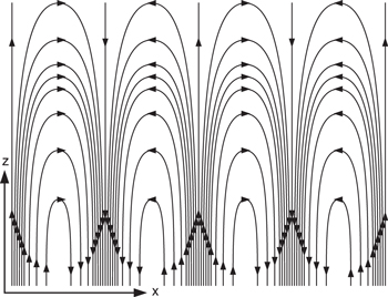
Zoom In Zoom Out Reset image size

It is easy to show that the combined current satisfies the conservation equation in equation (15). The conservation of the full topological charge current can be represented diagrammatically by continuous lines that represent the flow of topological charge. The one-dimensional initial topological charge density, considered here, gives rise to a two-dimensional topological charge flow diagram, as shown in figure 4. The diagram shows how, initially there is no transverse flow. Then the transverse flow gradually increases, reaching a maximum and then decreases again. At the same time the forward flow gradually decreases.

Zoom In Zoom Out Reset image size

It should be noted that the diagram in figure 4 does not represent the paths of actual optical vortices, but rather the average behavior of all the optical vortex distributions in the ensemble of stochastic optical fields for this case. Although the diagram is composed of discrete lines, the vector field that it represents is smooth and continuous over all points on the two-dimensional plane.

The dimension parameters need to ensure that certain conditions are satisfied. For the paraxial condition, we require that $\lambda {W}_{0}\ll 1$. It is also important that the scales over which the vortex distributions vary are much larger than the separation distance between adjacent vortices. For this condition we need to ensure that ${a}_{0}\ll {W}_{0}$ and ${b}_{0}\ll {W}_{0}$. We refer to this as the thermodynamic condition. Apart from these constraints on the dimension parameters in the one-dimensional case, the effect of varying the dimension parameters is merely a scaling of the functions in the transverse and longitudinal directions. The qualitative behavior of the topological charge current is unaffected by such variations in the dimension parameters.

For more complicated cases, such as the two-dimensional case, mentioned above, the phenomenology is much richer. There are more dimension parameters related to the shifts on the Fourier plane. As a result, qualitatively different kinds of behavior emerge, depending on the relative values of these shift parameters.

Knowledge of the transverse current completes the picture of how the topological charge distribution in a stochastic optical field evolves during propagation. The full topological charge current can now be computed for any monochromatic, paraxial normally distributed stochastic optical field. For the one-dimensional case considered here, the topological charge flow forms a fairly simple two-dimensional pattern. For more complex, two-dimensional initial topological charge distributions, the full topological charge current would be much more complex.

While the z-component of the topological charge current is the topological charge density, the transverse part is composed of quantities that are related to other quantities, such as the intensity or the phase gradient. As such the conservation equation provides a relationship among these quantities. It also related the rates of change in quantities along the propagation direction with rates of change in quantities along the transverse direction. In this sense the conservation equation serves as a predictive tool for the evolution of some quantities during propagation, based on the behavior of quantities on the transverse plane.

This conservation equation is akin to the intensity transport equation [19], which is also a conservation equation. It is expected that more such conservation equations can be obtained for quantities in stochastic optical field. Together, these equations would provide a better picture of the evolution of inhomogeneous stochastic optical fields.