

Abstract
In this communication, a novel technique to measure the temporal width of an ultra-short optical pulse using an electrically focus-tunable lens (EFTL) is proposed and implemented (no need for a mechanical translation stage). The principle is based on the time delay experienced by the pulse when it passes through the deformed membrane of the EFTL as the focal length changes by an applied current. The resolution of the system is approximately 0.23 fs, with a total time delay of 0.69 ps. A typical autocorrelation can be performed in less than 5 s with an excellent Signal to Noise Ratio. The same technique can be implemented to study ultrafast phenomena like electronic relaxation or ultrafast fluorescence in a pump-probe configuration.
Export citation and abstract BibTeX RIS
1. Introduction
In order to characterize ultrafast optical pulses with time-width less than 100 fs it is necessary to perform indirect measurements due to the lack of fast electronic devices capable of measuring pulses at that timescale [1]. Different optical methods have been proposed in order to overcome this limitation. For example, intensity autocorrelation [2] and interferometric autocorrelation [3, 4] methods are used when the shape of the intensity profile is known and only the time duration is of interest. However, if the shape of the pulse is unknown more sophisticated techniques are used in order to measure both amplitude and phase [5–7]. For example, one approach measures the frequency spectrum for each time delay, frequency resolved optical gating (FROG) [6], while a second approach analyses the spectral interference pattern of the two delay pulses, spectral phase interferometer for direct electric field reconstruction (SPIDER) [7]. One aspect that is common to all of these techniques is the need for a suitable optical delay line that converts the time resolution into a spatial resolution, which in general is accomplished by mechanical translation stages that most of the time are very costly, have limited time response, and might be a significant source of error if care is not taken [8]. Although this aspect has been tackled by different techniques [5, 9–13], most of them still rely on mechanical translation or rotational devices. In recent years different proposals to replace mechanical translation stages in optical setups by EFTL have been reported (e.g., M2 beam propagation factor measurement [14], confocal microscopy [15], self-interference digital holographic microscopy [16], retinal images [17], z-scan [18]). The goal is to reduce the complexity of the optical setup, the amount of mechanical components, the data collection time, and costs. Following this tendency, this work focused on reducing the complexity of autocorrelators that are based on mechanical translations, opening the possibility of more compact devices that can be built with less expensive equipment. To achieve this we have replaced the retroreflector and translation stage of the time-delay line of an intensity autocorrelation setup with an EFTL OPTOTUNE EL-10–30 lens. With the EFTL the time-delay is generated using the extra path length travel by the pulse as the lens changes its focal length.
In section two the difference between an intensity autocorrelation setup with a translation stage and our proposal is explained, together with the theoretical background that is needed. In section three the operation principle and characterization of the EFTL for its use in a delay line is presented. In section four the experimental setup for a mode-locked Ti:Sapphire laser is outlined, and in section five experimental results and conclusions are reported.
2. Modified intensity autocorrelation setup
2.1. Intensity autocorrelation with a translation stage
An Intensity autocorrelation function based on second harmonic generation (SHG) is a common method to measure the temporal duration, and to some extend the shape, of ultra-short optical pulses, and was introduced after the invention of the first mode-locked laser [19, 20] (a typical experimental setup is shown in figure 1). A laser beam pulse is divided by the beam splitter (BS) into two beams that are sent through the two arms of a modified Michelson interferometer. One of the beams is slow-frequency modulated and sent to the retroreflector RF-2 mounted on a mechanical translation stage with submicron spatial resolution. Later, both beams are recombined and focused by lens L1 on the nonlinear crystal NLC that generates in the bisecting direction of the two beams a second harmonic signal that corresponds to the second order correlation function given by:

where  is the intensity of the beam in the RF-1 arm and
  is the intensity of the beam traveling in the RF-2 arm,
  is time, and
  is the time-delay. The signal
  is integrated by the slow detector D and sent to a lock-in amplifier connected to a computer were the data points for all the time-delays are recorded. In the above equation τ is the time-delay between the two pulses controlled with the mechanical translation stage by increasing or decreasing the optical path length of the RF-2 arm. To obtain the beam pulse time duration the correlation function width is multiply by a factor that depends on the pulse shape (1.543 for our case of a sech2 pulse shape).
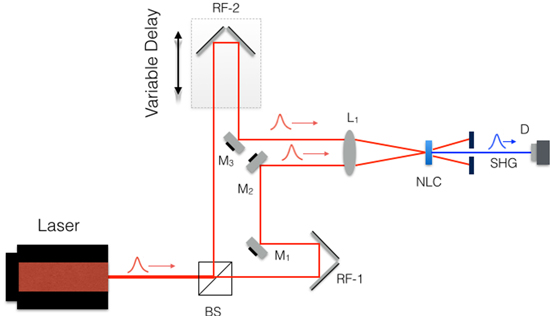
Figure 1. Experimental setup for the intensity autocorrelation base on second harmonic generation: mechanical translation stage. BS: beam splitter, M: mirror, NLC: nonlinear crystal, RF: retroreflector, D: detector, L: lens.
Download figure:
Standard image High-resolution image2.2. Intensity autocorrelation with an EFTL
When the retroreflector and translation stage are replaced by an EFTL the optical setup in figure 1 is replaced by the optical setup shown in figure 2. In this case the time-delay is generated by using the extra path length travel by the pulse as the EFTL lens changes its focal length. In figure 2 a laser beam pulse is divided by the BS into two beams. One of the beams, slow-frequency modulated, is sent to the EFTL while the other beam is sent to the lens L1. Both beams are focused by each lens respectively, and recombined on the nonlinear crystal NLC generating the second harmonic signal. For this case the corresponding second order correlation function is given by:

where  is the intensity of the fixed-focal length lens beam and
  is the intensity of the EFTL beam. In equation (2) the intensity of the EFTL must be modified to include intensity variations due to the variation of the beam radius at the SHG crystal, because the focal distance of the EFTL is changing. Therefore, the SHG signal is the result of the temporal as well as the spatial overlap of the two beams, and it is necessary to take into account that the intensity of the SHG is modified by the focus/defocus of the EFTL. This can be accomplished (assuming that the spatial intensity profile of the beam is Gaussian) by calculating the fraction of the power carried by the beam within a circle of radius ρo corresponding to the fixed-focal length lens beam, which is given by:

where P is the total beam power, and  is the beam radius of the EFTL at the sample. This radius depends on the sample distance from the EFTL, d, and the focal length of the EFTL through the expression:

where

Then, the intensity of the EFTL beam can be written as:

It is important to determine the relation between the fixed-focal length spot size and the spot size of the EFTL at the sample, such that the autocorrelation is dominated by SHG and not by focus/defocus of the EFTL. We have performed numerical simulations involving equations (2) and (3) for different pulse durations and have found that if the condition in equation (7) is met the autocorrelation will be dominated by temporal delay of the beam and will represent a real autocorrelation.

where  is the pulse temporal duration.
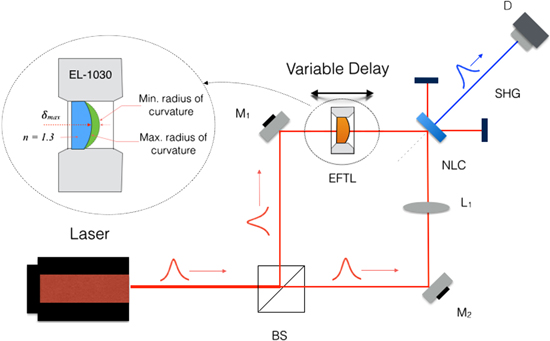
Figure 2. Experimental setup for the intensity autocorrelation base on second harmonic generation: BS—beam splitter, M1 and M2 are mirrors, L1: fixed-focal length lens, EFTL: electrically focus-tunable lens, SHG: second harmonic signal and D: detector. Inset: EFTL Optorune EL-1030.
Download figure:
Standard image High-resolution image3. Operation principle and lens characterization
Our experimental technique is based on the extra path length travel by the pulse as the EFTL changes its focal length. This type of lens changes its shape (curvature) due to an optical fluid sealed off by a polymer membrane. When the ring of the membrane is squeezed by an electromagnetic actuator the liquid is forced into the central portion of the lens, which causes the membrane to bulge and as a consequence the focal length changes; whence, the displacement of the center of the EFTL membrane is a function of the applied current. The maximum current and minimum current passing through the lens corresponds to the minimum and maximum focal length, respectively. The current range is from 0 to 300 mA with a resolution given by the manufacturer of 0.1 mA, with a maximum membrane displacement of δmax = 0.73 mm.
To make use of the extra path length the focal length of the EFTL has to be correctly characterized as a function of the applied current. To achieve this we used an open-aperture f-scan configuration with a CdS crystal sample [21]. By finding the minimum in the open-aperture setup for two different sample-lens separations the focal length-current relation can be fitted to:

where  is the current passing through the lens in mA and
  is the focal length in centimeter.
The beam waist radius at the focus of the lens as a function of focal length was measured with a laser beam profiler and it was found to obey in good approximation the relation:

where  is the wavelength of the pulse,
  is the laser beam diameter at the entrance surface of the lens, and
  is a correction factor due to the fact that the EFTL is not a perfect spherical lens.
To calibrate the time scale as a function of current,

where  is the speed of light and
  is the displacement of the central portion of the lens as a function of current. Thus, for a reported refractive index inside the lens of
  at 800 nm the maximum expected time-delay is 0.73 ps with a resolution of 0.24 fs. In order to verify this result we recorded the mechanical intensity autocorrelation of the pulse for various currents at increments of 20 mA (figure 3). Then we measured the time-delay and plotted it as a function of the applied current, as shown in figure 4. The experimental data verifies the linear response of the EFTL within the experimental error.
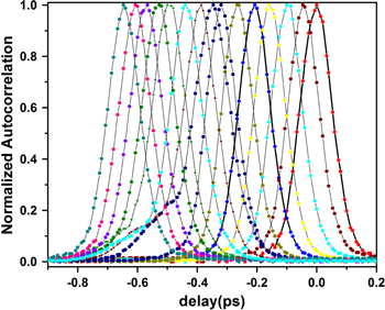
Figure 3. Mechanical autocorrelation of the pulse for currents between 0 mA (trace centered at 0.0 ps) and 280 mA (trace centered at −0.65 ps), at increments of 20 mA.
Download figure:
Standard image High-resolution image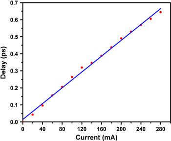
Figure 4. Pulse delay as a function of the applied current between 0 mA and 280 mA, at increments of 20 mA. (dots) experimental data; (continuous line) linear fit.
Download figure:
Standard image High-resolution imageFrom the linear fit the time-delay produced by the deformation of the lens membrane can be approximated to a linear response of the form

This allows a total experimental displacement of 0.69 mm for the entire current range, which is in good agreement with the value given by the manufacturer. Thus, our EFTL lens is found to be able to generate an approximate time-delay of 2.3 fs mA−1 with a total delay of 0.69 ps.
4. Experimental setup
Our experimental setup is shown in figure 2. In this setup the original pulse is generated by a mode-locked Ti:Sapphire laser which is capable of generating sub 100 fs pulses with a repetition rate of 90.9 MHz. After the BS the two beams are redirected towards a BBO crystal by mirrors M1 and M2. One of the beams passes through a fixed-focal length lens with focal distance equal to 12 cm and the second beam passes through the EFTL.
The EFTL is controlled by an OPTOTUNE lens driver, which gives a full current range from 0 to 300 mA with a reported resolution of 0.1 mA. The two beams are then recombined inside a BBO crystal (angle phase match). The generated second harmonic signal is detected by a Si-photodetector and a STANFORD RESEARCH 830 dual channel Lock-in amplifier, controlled through a GPIB interface. For our experiment 

 and
and  .
.
A critical aspect of the experimental implementation of this technique is the correct alignment of the beam as it passes through the optical axis of the EFTL. This is necessary in order to use the maximum δmax of the membrane and to prevent the beam that goes through the EFTL from changing location at the overlapping spot plane as the focal length changes.
It is important to point out that because of the simplicity of the setup and the absence of retroreflectors, fine-tuning of the setup can easily be accomplished. First performing by hand a coarse temporal alignment of the pulses, giving an optical path difference between the two arms of the autocorrelator to better than 1 cm of accuracy. The fine-tuning is achieved adjusting the EFTL arm with a XYZ-translation stage of standard micrometer sensitivity and 4 cm of translation range.
To estimate the dispersion mismatch in the two arms because of the difference in the refractive index, for regular lenses (BK7 ∼ 1.51 at 780 nm, and group velocity dispersion GVD = 36.16 fs2 mm−1) we found that for the fixed-focal length lens of 5 mm thickness at the center, a 80 fs pulse will experience a pulse broadening of 0.2 fs, which is negligible for the type of pulses that we are measuring. In the case of an EFTL with 5 mm thickness and refractive index variation as shown in figure 5 [20], the GVD = 27.7 fs2 mm−1 and the pulse broadening is 0.08 fs. Therefore, we can say that the effect of the lens in the pulse broadening can be ignored. In addition, from figure 5 one can observed that the variation of n for wavelengths ranging from 486 to 1550 nm is of the order of 1%. Thus, the EFTL can be considered, to a good approximation, as achromatic.
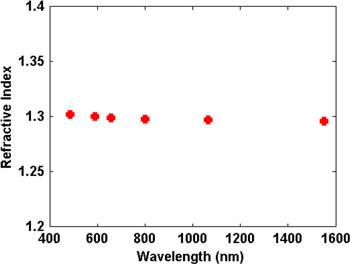
Figure 5. Refractive index of EFTL as a function of wavelength.
Download figure:
Standard image High-resolution imageFrom figure 2 is clear that the experimental setup shown in figure 1 has been reduced considerably not only in complexity and number of optical components but most importantly, in cost.
5. Experimental results
A typical trace of the autocorrelation as a function of current is shown in figure 6; it is worth mentioning that this trace can be acquired in less than 5 s depending on the driving electronics operating the EFTL.

Figure 6. A normalized autocorrelation trace as a function of current, by using the EFTL.
Download figure:
Standard image High-resolution imageTo transform the current scale into a time delay in the trace shown in figure 6, we multiply the current values by the factor 2.3 fs mA−1 that was found experimentally. The maximum SHG occurs at zero time delay. In our case this corresponds to an EFTL focal length of 13.3 cm (the distance between the BBO crystal and the EFTL), produced when the EFTL current is 127 mA.
To verify the accuracy of the method we performed a mechanical intensity autocorrelation and an EFTL intensity autocorrelation (figure 7). The data show a remarkable agreement given the fact that there are no fitting parameters. Each one of the traces gives a value of 126 fs (at FWHM) for the width of the intensity autocorrelation, which corresponds to 81 fs (at FWHM) for pulse duration. Notice that the tail at the low current setting of the EFTL-AC or positive delay time can be attributed to the fact that for low currents the focal length is large and the condition given by equation (7) is not completely fulfill and therefore the signal intensity has an important defocusing dependency, yet the pulse width can be determined correctly.
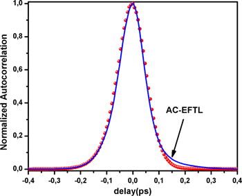
Figure 7. Mechanical intensity autocorrelation (dots) and EFTL intensity autocorrelation (AC-EFTL) (continuous line). Both traces give an autocorrelation time-width of 47 fs.
Download figure:
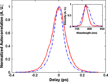
Standard image High-resolution imageFinally, we have modified the spectral-bandwidth of the pulse by introducing more dispersion with the intracavity-compensation prism of the laser. As a result, a spectral narrowing of the pulse is generated and therefore an increase in the pulse temporal duration (due to the extra GVD experienced by the pulse in the intracavity). The autocorrelation for both cases is shown in figure 8, and the spectral broadening in figure 8 (inset). It is evident that the pulse temporal broadening is captured by the EFTL, which can be used as convincing evidence that it is dominated by temporal delay and not by focusing/defocusing of the EFTL.
Figure 8. EFTL intensity autocorrelation for (continuous line) short-bandwidth and (dashed line) large bandwidth. Inset: normalized spectral density as a function of wavelength for (continuous line) short-bandwidth and (dashed line) large bandwidth.
Download figure:
Standard image High-resolution image
In conclusion, we have performed an intensity autocorrelation of an ultra-short pulse generated by a Ti:Sapphire laser by using a simple low-cost EFTL, and found excellent agreement with the pulse width obtained with a mechanical intensity autocorrelation. This is a low cost setup that can be used for pulse characterization and even for pump-probe experiments where the dynamics of the system is in the sub-ps regimen. In order to represent a real autocorrelation it is critical to make the spot size of the beam produced by the fixed focal-length lens  greater than the beam produced by the EFTL. This work has focused on reducing the complexity of autocorrelators that are based on mechanical translations, opening the possibility of less expensive systems.
HG acknowledges support by the NSF through grant CMMI-0757547, and the support by the Fulbright program for international exchange. JS acknowledges financial support by COLCIENCIAS. ER and JS acknowledge financial support by Estrategia de Sostenibilidad 2014-2015 de la Universidad de Antioquia and thanks to the Universidad de Antioquia.