

Abstract
This paper assesses the effect of thermal stratification on the prediction of inert tracer gas dispersion within a cavity of height (H) 1.0 m, and unity aspect ratio, using large eddy simulation. The Reynolds number of the cavity flow, was 67 000. Thermal stratification was achieved through the heating or cooling of one or more of the walls within the cavity. When compared to an isothermal (neutral) case, unstable stratification from surface heating generally has a weak influence on the primary recirculating cavity vortex, except in the case where the windward wall is heated. For windward wall heating, a large secondary vortex appears at the corner of the windward wall and cavity floor. Unstable stratification has no significant influence on the removal of pollutant mass from the cavity. Stable stratification through surface cooling drastically alters the flow pattern within the cavity, pushing the cavity vortex towards the upper quadrant of the cavity. As a result, large regions of stagnant fluid are present within the cavity, reducing the effectiveness of the shear layer at removing pollutant concentration from the cavity. Some stable stratification configurations can increase the pollutant mass within the cavity by over a factor of five, when compared to the neutral case. Pollutant concentration flux maps show that, in stably stratified cases, the majority of pollutant transport from the cavity is the result of entrainment into the primary cavity vortex. The results show that pollutant concentrations in urban street canyon-type flows are substantially altered by diurnal heating and cooling, which may influence pedestrian management strategies in urban environments.
Export citation and abstract BibTeX RIS

Original content from this work may be used under the terms of the Creative Commons Attribution 4.0 license. Any further distribution of this work must maintain attribution to the author(s) and the title of the work, journal citation and DOI.
Recommended by Professor Hyung Jin Sung
1. Introduction
A shear-driven cavity flow is a canonical flow type, with relevance to a wide range of practical configurations. The shear layer which evolves over the top of the cavity is responsible for the entrainment of freestream fluid into the cavity, and the removal of any contaminants present in it. Extensive research over the last 50 years has shown that shear layers contain large-scale coherent structures embedded within the turbulent flow (Brown and Roshko 1974, Winant and Browand 1974), which play a crucial role in the mixing of fluid within the shear layer (Koochesfahani and Dimotakis 1986, Karasso and Mungal 1996, Pickett and Ghandhi 2002). Urban street canyon (USC) flows, which can be approximated as a flow within a cavity, are the subject of intensive research, owing to the need to mitigate against vehicular pollution in city streets. As over 50% of the human population lives in urban areas (Department of Economic and Social Affairs 2014), there is an obvious need to reduce the effect of air pollution in urban environments (Burnett et al 2000, Cohen et al 2005).
There exists a range of factors which can influence the flow within a cavity. The Reynolds number of the cavity flow, based on the freestream velocity and the cavity height, affects the large-scale vortex structure within the cavity. The flow has been shown to be Reynolds number independent above a critical value (Snyder 1972, Uehara et al
2000, Allegrini et al
2013), although some doubts still remain as to whether any proposed critical value is truly universal (Chew et al
2018). The aspect ratio of the cavity height, H, to the cavity width, W, can be used to delineate the flow into three distinct regimes: skimming flow for  , wake interference flow for
  , and isolated roughness flow for
  (Oke 1988). Finally, the heating or cooling of solid walls within the cavity can influence the flow field, commonly referred to as thermal stratification effects (Nakamura and Oke 1988). Stable stratification is where the ambient air is warmer than surrounding walls, and unstable stratification is where the ambient air is cooler than the surrounding walls. Diurnal cycles of heating and cooling in urban street canyons can have a marked effect on the dispersion of pollutants within them (Kovar-Panskus et al
2002, Xie et al
2007). It is the final parameter, thermal stratification, which is the subject of the present study.
(Oke 1988). Finally, the heating or cooling of solid walls within the cavity can influence the flow field, commonly referred to as thermal stratification effects (Nakamura and Oke 1988). Stable stratification is where the ambient air is warmer than surrounding walls, and unstable stratification is where the ambient air is cooler than the surrounding walls. Diurnal cycles of heating and cooling in urban street canyons can have a marked effect on the dispersion of pollutants within them (Kovar-Panskus et al
2002, Xie et al
2007). It is the final parameter, thermal stratification, which is the subject of the present study.
Experimental measurements in real-world USCs are challenging, owing to the natural variation in local climactic conditions (DePaul and Sheih 1986, Fernando 2010, Dallman et al 2014). Experiments are therefore typically conducted at laboratory scale, where conditions can be more readily controlled. The majority of published experimental research on USCs deals with neutral conditions (i.e. isothermal flow) (Gerdes and Olivari 1999, Pavageau and Schatzmann 1999, Baik et al 2000, Salizzoni et al 2009, Kikumoto and Ooka 2018), with fewer papers dealing with stable stratification (Uehara et al 2000), and unstable stratification conditions (Uehara et al 2000, Kovar-Panskus et al 2002, Kim and Baik 2005, Allegrini et al 2013). To produce stratified conditions in laboratory experiments, it is common practice to heat (or cool) walls in the cavity to a constant temperature, which can cause difficulties in ensuring consistency of the wall temperature (Allegrini et al 2013).
Numerical simulation techniques have become an increasingly popular method to study contaminant dispersion in cavities over the last 25 years. Reynolds-averaged Navier Stokes (RANS) methods have been applied to cavity flows for both neutral (Sini et al 1996, Baik and Kim 1999), and stratified flow conditions (Li et al 2006, Xie et al 2006, Hang et al 2016), with reasonable results obtained. RANS methods model all turbulent scales of motion in the flow, which leads to inherent inaccuracies in the solutions owing to the fact that the turbulent eddies responsible for the transport of mass and momentum are absent from the RANS solution. Large eddy simulation (LES) has been recognised as a valuable tool for the study of cavity flows as the large-scale motions responsible for the transport of the contaminant in the flow are resolved explicitly. LES permits the study of high Reynolds number flows which are not currently tractable using direct numerical simulation, but the removal of small scales below a characteristic filter width introduces the requirement of subgrid-scale modelling to close the LES equations. Many such models exist in the literature, with the Smagorinsky model (Smagorinsky 1963), the WALE model (Nicoud and Ducros 1999), and the Germano–Lilly model (Germano et al 1991, Lilly 1992), being the most commonly used for USC/cavity flows (Tominaga et al 2008, Cheng and Liu 2011, Kikumoto and Ooka 2018). LES has been extensively used to simulate cavity-type flows at isothermal conditions (Li et al 2009, Han et al 2018, Kikumoto and Ooka 2018, McMullan 2022), where it has been shown that the vortex structure within the cavity is captured using LES (Cui et al 2004), and that the aspect ratio of the cavity plays a key role in the topology of the vortex structure within it (Li et al 2008). LES studies of the cavity-type flow at thermally stratified conditions are less common in the literature, with both unstable stratification conditions (Li et al 2010, Park et al 2012), and stable stratification conditions considered (Li et al 2015, 2016). Unstable stratification is typically produced in LES through assigning an elevated temperature boundary condition to the floor of the cavity, with respect to the ambient flow temperature (Li et al 2010), with stable stratification achieved through assigning temperature values to the floor which are lower than the ambient (Li et al 2015, 2016). Further studies have considered the effect of heating the other individual walls in the cavity (Xie et al 2007, Park et al 2012), but no published research to date has studied the Reynolds number independent thermally stratified flow, where individual walls are heated or cooled.
In this research, the effects of thermal stratification on the dispersion of tracer gas within a simulated laboratory-scale cavity are studied. The numerical simulations are based on the isothermal experiments of Kikumoto and Ooka (2018), and a validated OpenFOAM LES method is used to perform the simulations (McMullan 2022). The effects of thermal stratification are assessed through the heating of walls within the cavity to produce unstable stratification, or cooling of the walls within the cavity to produce stable stratification. Comparisons of the stratified flow fields with the isothermal flow will be made to highlight key changes to the mechanisms through which the tracer gas is transported around the cavity, and subsequently removed from it by the cavity shear layer. Concentration probability density functions (PDFs) are produced, which demonstrate how surface heating or cooling can influence the predicted range of concentrations of a contaminant in the cavity.
This paper is organised as follows. The numerical methods employed in the research are described in section 2. The setup of the simulations is outlined in section 3. The influence of stratification on the flow-field within the cavity is discussed in section 4. The dependence of the tracer gas dispersion on the stratified cavity flow is presented in section 5. Concluding remarks are provided in section 6.
2. Numerical methods
In OpenFOAM LES, an implicit spatial filtering process removes the unresolved scales of motion from the flow, and introduces a subgrid-scale stress tensor, τij
=  into the filtered momentum equation, where
  is the filtered velocity field. Invoking the Boussinesq approximation to account for the buoyancy force generated by changes in temperature in the fluid leads to the governing equations for an incompressible, buoyant flow:


where ρ0 is the reference density, ρ is the effective density, p is the pressure, g is gravitational acceleration,  is the spatially-filtered temperature,
  is a reference temperature, β is the thermal expansion coefficient of the fluid, and the Kronecker delta,
  , has a value of unity in the vertical direction.
The transport equation for the spatially-filtered temperature field is given by

where  is the thermal diffusivity. In LES, the thermal diffusivity
  is the sum of the resolved and subgrid-scale components,
  . The resolved component is modelled through
  , and the subgrid-scale component is computed through
  , where Pr is the Prandtl number,
  is the turbulent Prandtl number, and
  is the subgrid kinematic viscosity. For the present simulations, Pr = 0.7, and
  = 0.85.
The filtered scalar transport equation is given by

where  is the filtered scalar, αξ
is the scalar diffusivity, and
is the filtered scalar, αξ
is the scalar diffusivity, and  is a source term. Similar to the temperature transport equation, the scalar diffusivity
  is the sum of the molecular diffusivity and the subgrid diffusivity,
  , with the molecular and subgrid diffusivities modelled by a gradient-diffusion approach, such that
  , and
, and  , where Sc is the Schmidt number, and
  is the turbulent Schmidt number. In this study, Sc = 1, and
  = 0.5, following previous numerical studies of pollutant dispersion in a cavity (Kikumoto and Ooka 2018, McMullan 2022).
In LES, a subgrid scale model is required to close the filtered equations above. For incompressible flows, a common approach to modelling the SGS tensor is through

where  is the strain rate tensor and δij
is the Kronecker delta. Many subgrid scale models exist in the literature, and previous studies of tracer gas dispersion in an isothermal cavity flow have shown that the WALE model produces highly accurate results for both the predicted velocity field, and for the tracer gas concentration statistics (McMullan 2022). In the WALE model (Nicoud and Ducros 1999), the subgrid viscosity is evaluated through
is the strain rate tensor and δij
is the Kronecker delta. Many subgrid scale models exist in the literature, and previous studies of tracer gas dispersion in an isothermal cavity flow have shown that the WALE model produces highly accurate results for both the predicted velocity field, and for the tracer gas concentration statistics (McMullan 2022). In the WALE model (Nicoud and Ducros 1999), the subgrid viscosity is evaluated through
where  ,
,  , and
, and  .
.
The LES results reported here are performed using the OpenFOAM v2112 solver suite (www.openfoam.com). The open-source CFD software suite has been used extensively in the study of urban environment flows (Jeanjean et al 2015, Zhong et al 2015, García-Sánchez et al 2018, Kikumoto and Ooka 2018, McMullan 2022, McMullan and Angelino 2022). The filtered variables are stored on a collocated grid, and the governing equations are solved using a PIMPLE algorithm. Time advancement is achieved through a second-order accurate upwind Euler scheme. Second-order central-differencing schemes are used in the solution of the momentum equation, and a total variation diminishing (TVD) scheme is used for the advective terms in both the scalar transport equation, and the temperature transport equation. The TVD scheme minimises out of bounds errors for the scalar and temperature fields (Yee 1987, Dianat et al 2006).
3. Simulation setup
The simulations are based on the experimental research of Kikumoto and Ooka (2018). The experiment studied the dispersion of ethylene tracer gas within a laboratory-scale cavity, at isothermal conditions. The cavity had dimensions of  in the streamwise (x), vertical
  ), and spanwise (z) directions respectively, where the cavity height H = 1 m. These dimensions result in the flow being of the skimming type, as defined in section 1. At the top of the cavity, channels of dimensions
  provided the inlet and outlet channels to the experiment. A line source was placed in the middle of the cavity floor, which emitted the ethylene tracer gas at a rate of 3.0 l min−1. The inflow velocity of air into the rig was 1.0 ms−1, with a turbulence intensity of 4%. The Reynolds number of the experiment, based on the inflow velocity and the cavity height, was 67 000, far in excess of the values assumed to denote Reynolds number independence in a cavity with unity aspect ratio, reported as
  11 000 (Chew et al
2018), and
11 000 (Chew et al
2018), and  13 000 (Allegrini et al
2013). The boundary layer at the upstream edge of the cavity was assumed to be laminar. All measurements were recorded at mid-span of the rig,
13 000 (Allegrini et al
2013). The boundary layer at the upstream edge of the cavity was assumed to be laminar. All measurements were recorded at mid-span of the rig,  .
.
The computational domain shown in figure 1 used in the current study is a numerical recreation of the experimental geometry. Extensive numerical validation studies have been performed against the isothermal reference dataset (Kikumoto and Ooka 2018, McMullan 2022). It has been shown that a uniform grid-spacing of  yields highly accurate predictions of both the velocity statistics, and the tracer gas concentration statistics (McMullan 2022). It has also been shown that the WALE model (Nicoud and Ducros 1999), and Germano–Lilly subgrid-scale model (Germano et al
1991, Lilly 1992), produce more accurate flow statistics at this grid resolution (McMullan 2022), when compared to the standard Smagorinsky model (Smagorinsky 1963). Owing to the above findings, the present study uses a grid with spacings of
yields highly accurate predictions of both the velocity statistics, and the tracer gas concentration statistics (McMullan 2022). It has also been shown that the WALE model (Nicoud and Ducros 1999), and Germano–Lilly subgrid-scale model (Germano et al
1991, Lilly 1992), produce more accurate flow statistics at this grid resolution (McMullan 2022), when compared to the standard Smagorinsky model (Smagorinsky 1963). Owing to the above findings, the present study uses a grid with spacings of  in each direction, and employs the WALE model with model coefficient
  . The domain is discretised by 27.648 million cells, and the near-wall resolution, expressed in non-dimensional units, is
  inside the cavity.

Figure 1. Schematic of the computational domain, based on the reference experiment (Kikumoto and Ooka 2018). Black circles in the diagram denote the locations of experimental measurement locations. All measurements were recorded at mid-span,  0.15.
0.15.
Download figure:
Standard image High-resolution imageA uniform streamwise velocity profile of  ms−1 is imposed as the inflow boundary condition, onto which pseudo-random disturbances of magnitude 4%
  in the x-direction, and 2%
  in the y- and z-directions, are superimposed at each time step. The concentration of the transported scalar is zero at the inflow boundary. For these inflow conditions, the boundary layer at the upstream cavity edge is laminar in nature, and has a momentum thickness,
  m, for all simulations. A zero-gradient condition is applied to the outflow boundary for both the velocity and scalar fields. The walls of the cavity, including the spanwise walls, are solid boundaries which are modelled as a no-slip boundary condition for the velocity field, and a zero-gradient condition for the scalar field. In all simulations the tracer gas line source is modelled as an inflow boundary condition at the centre of the cavity floor with a constant vertical velocity of 0.01923 ms−1, yielding a constant flux. The passive scalar is assigned a value of unity at the line source boundary.
To study the effects of thermal stratification, walls within the cavity are either heated to produce an unstably stratified flow, or cooled to produce a stably stratified flow. The Richardson number of the flow (Park et al 2012) is defined as

where Tn
is the fluid temperature at  ,
,  is the temperature of the heated wall(s) in the cavity, and Un
is the mean streamwise velocity at
is the temperature of the heated wall(s) in the cavity, and Un
is the mean streamwise velocity at  .
.
For flows with unstable stratification, the freestream air has a temperature of 293 K, and walls which are heated are assigned a constant temperature boundary condition of 318 K. For stable stratification, the freestream air has a temperature of 318 K, and the walls which are cooled are assigned a constant temperature of 293 K. Walls which are neither heated nor cooled in each simulation are assigned a zero-gradient temperature boundary condition, and a similar condition is applied to the outflow boundary. The Richardson numbers of all simulations considered in this study are given in table 1. In all stratified simulations, the tracer gas emitted from the line source is assigned a temperature of 305.5 K.
Table 1. Richardson number, Rb , of the simulations.
| Case | Configuration | Rb |
|---|---|---|
| N | Isothermal | 0 |
| U-A | Leeward wall heating | −1.29 |
| U-B | Ground heating | −1.35 |
| U-C | Windward wall heating | −1.41 |
| U-All | All walls heated | −1.28 |
| S-A | Leeward wall cooling | 1.35 |
| S-B | Ground cooling | 1.34 |
| S-C | Windward wall cooling | 1.37 |
| S-All | All walls cooled | 1.37 |
The time step in each simulation is  s, which maintained the CFL number below unity. Once the flow attained a statistically stationary state, flow statistics are gathered for a duration of 360 s. Velocity and concentration probe data are recorded at all 18 locations shown in figure 1, at a rate of 1 kHz. Velocity statistics are normalised by Un
, and concentration statistics are normalised by a reference concentration,
s, which maintained the CFL number below unity. Once the flow attained a statistically stationary state, flow statistics are gathered for a duration of 360 s. Velocity and concentration probe data are recorded at all 18 locations shown in figure 1, at a rate of 1 kHz. Velocity statistics are normalised by Un
, and concentration statistics are normalised by a reference concentration,  , where
  is the emission rate of the tracer gas, and
  . All statistics presented here are recorded along the mid-span of the computational domain
  . Each simulation had a run time of 200 h, parallelised over 32 Intel Xeon 2.4 GHz, 14-core CPUs.
A naming convention is established whereby the walls of the cavity are assigned labels, as shown in figure 1, i.e. for an unstably stratified flow with ground heating, the simulation is denoted U-B. Similarly, for stable stratification with all walls cooled, the simulation is denoted S-All. Case N refers to a simulation performed at neutral (isothermal) conditions.
4. Flow statistics
Figure 2 shows the mean streamlines of the flow for all simulations, coloured by the normalised mean velocity magnitude,  , where U and V are the mean streamwise velocity, and the mean vertical velocity, respectively.

Figure 2. Streamlines of the mean velocity field at mid-span of the cavity. Streamlines are coloured by the normalised mean velocity magnitude.
Download figure:
Standard image High-resolution imageThe neutral case contains a primary recirculation vortex in the cavity, which has a clockwise rotational sense. In addition, there are three corner vortices — two of which are found in the corners on the floor of the cavity, and one immediately below the top of the cavity on the leeward wall. For the unstably stratified cases, heating of the leeward wall in simulations U-A and U-All removes the small vortex immediately below the top of the cavity on this wall. The vortex at the corner of the floor and the windward wall is absent in U-A, and U-B. In U-C a large secondary vortex is present in the corner of the floor and the heated windward wall. With the exception of U-C, all unstably stratified cases show an increase in the magnitude of the circulation velocity of the large central vortex, in agreement with previous experimental studies of the unstably stratified flow (Allegrini et al 2013).
The streamlines for the stably stratified cases show that surface cooling has a significant impact on the flow within the cavity, with the flow field noticeably different from that of the unstably stratified cases. In simulations S-A, S-C, and S-All, the primary cavity vortex moves towards the upper windward quadrant of the cavity, with the flow in the remainder of the cavity appearing to be relatively stagnant. In the region of  , each of these three simulations show sharp curvature in the mean streamlines, which suggests that highly turbulent flow activity is occurring in the region of the cavity shear layer. For the case with floor cooling, S-B, the streamline pattern bears some resemblance to the isothermal case in that a large vortex occupies most of the cavity, with the centre of rotation of the vortex pushed towards the windward wall. The streamline pattern in the
  simulations bears close qualitative resemblance to experiments of stably stratified flows (Uehara et al
2000). The centre of rotation of the primary cavity vortex in each simulation is outlined in table 2, along with the percentage shift in the location of the vortex with respect to case N. In all unstably stratified simulations, there are only slight changes in the location of the cavity vortex when compared to the neutral case. In the stable stratification simulations, it is only in case S-B that the primary vortex resides near to mid-height of the cavity — in other cases, the primary recirculation vortex resides far into the upper windward quadrant of the cavity.
simulations bears close qualitative resemblance to experiments of stably stratified flows (Uehara et al
2000). The centre of rotation of the primary cavity vortex in each simulation is outlined in table 2, along with the percentage shift in the location of the vortex with respect to case N. In all unstably stratified simulations, there are only slight changes in the location of the cavity vortex when compared to the neutral case. In the stable stratification simulations, it is only in case S-B that the primary vortex resides near to mid-height of the cavity — in other cases, the primary recirculation vortex resides far into the upper windward quadrant of the cavity.
Table 2. Location of centre of rotation of the cavity vortex in all simulations. Percentage shift in each direction corresponds to the change in location of the cavity vortex centre of rotation, with respect to the neutral case N.
| Case |

| % x-shift | % y-shift |
|---|---|---|---|
| N | 0.551, 0.502 | — | — |
| U-A | 0.554, 0.521 | 0.5 | 3.8 |
| U-B | 0.532, 0.510 | −3.4 | 1.6 |
| U-C | 0.536, 0.594 | −2.7 | 18.3 |
| U-All | 0.532, 0.540 | −3.4 | 7.6 |
| S-A | 0.774, 0.758 | 40.5 | 51.0 |
| S-B | 0.647, 0.532 | 17.4 | 6.0 |
| S-C | 0.841, 0.832 | 52.6 | 65.7 |
| S-All | 0.848, 0.848 | 53.9 | 68.9 |
Profiles of the mean streamwise velocity recorded at  are shown in figure 3(a) for the unstable stratification simulations, along with the neutral simulation (McMullan 2022), the neutral experimental data (Kikumoto and Ooka 2018), and experimental data for an unstably stratified flow with ground heating (Uehara et al
2000). It is important to note that the unstably stratified experimental data is provided for qualitative comparison with U-B only, as the experimental configuration comprised a cubic array of model buildings with ground heating, rather than the single cavity considered here. In case U-C, the large secondary vortex in the corner of the floor and windward wall serves to reduce the magnitude of the recirculation velocity at the floor, while the other cases show an increase in the circulation velocity in the vicinity of both the floor and the top of the cavity. The velocity profile in the region of the cavity shear layer shows that there is a slight thickening of the layer in U-A, U-B, and U-All. Comparison of U-B with the data of Uehara et al (2000) suggests that the effects of ground heating on the flow in the cavity have been captured appropriately. The root mean squared (r.m.s.) streamwise velocity fluctuation profiles at
are shown in figure 3(a) for the unstable stratification simulations, along with the neutral simulation (McMullan 2022), the neutral experimental data (Kikumoto and Ooka 2018), and experimental data for an unstably stratified flow with ground heating (Uehara et al
2000). It is important to note that the unstably stratified experimental data is provided for qualitative comparison with U-B only, as the experimental configuration comprised a cubic array of model buildings with ground heating, rather than the single cavity considered here. In case U-C, the large secondary vortex in the corner of the floor and windward wall serves to reduce the magnitude of the recirculation velocity at the floor, while the other cases show an increase in the circulation velocity in the vicinity of both the floor and the top of the cavity. The velocity profile in the region of the cavity shear layer shows that there is a slight thickening of the layer in U-A, U-B, and U-All. Comparison of U-B with the data of Uehara et al (2000) suggests that the effects of ground heating on the flow in the cavity have been captured appropriately. The root mean squared (r.m.s.) streamwise velocity fluctuation profiles at  are shown in figure 3(b). There is a general increase in the magnitude of the fluctuations within the cavity, for all cases where one or more walls are heated.

Figure 3. Normalised velocity statistics from the unstably stratified simulations, obtained at  0.5. Case N, and experimental data, recorded at isothermal conditions.
Download figure:
Standard image High-resolution imageThe mean streamwise velocity profiles recorded at  in the stable stratification simulations are shown in figure 4(a). Stably stratified experimental data for a case with ground cooling is also shown on this plot (Uehara et al
2000) to provide a qualitative comparison for simulation S-B. The reason why only a qualitative comparison can be made for case S-B is the same as that outlined in the previous paragraph for case U-B. The presence of a large cavity vortex in S-B results in some recirculation of flow along the floor of the cavity, providing a reasonable comparison to the stably stratified experimental data. In all of the other
in the stable stratification simulations are shown in figure 4(a). Stably stratified experimental data for a case with ground cooling is also shown on this plot (Uehara et al
2000) to provide a qualitative comparison for simulation S-B. The reason why only a qualitative comparison can be made for case S-B is the same as that outlined in the previous paragraph for case U-B. The presence of a large cavity vortex in S-B results in some recirculation of flow along the floor of the cavity, providing a reasonable comparison to the stably stratified experimental data. In all of the other  simulations, however, the fluid is effectively stagnant over the lower 50% of the cavity height. The associated r.m.s. streamwise velocity fluctuation profiles, shown in figure 4(b), are also negligible in this region. For S-A a pronounced peak in the
  profile is observed in the region of
  , which is caused by the interaction of the primary recirculation vortex with the stagnant fluid in the cavity. The width of the peak in the profile caused by the cavity shear layer is substantially greater in the stably stratified simulations, suggesting that the growth of the shear layer is more rapid in these cases.
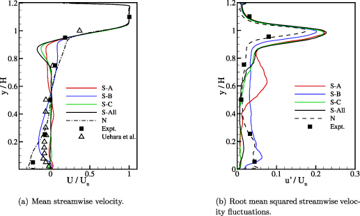
Figure 4. Normalised velocity statistics from the stably stratified simulations, obtained at  0.5. Case N, and experimental data, recorded at isothermal conditions.
Download figure:
Standard image High-resolution imageFigure 5 shows profiles of the normalised mean vertical velocity, recorded at mid-height,  , of the cavity. With the exception of U-C, the action of heating the cavity wall(s) in the unstably stratified cases is to increase the magnitude of the updraft (positive vertical velocity) at the leeward wall, and the magnitude of the downdraft (negative vertical velocity) at the windward wall, with respect to the neutral experiment and simulation. In case U-C, the magnitude of the updraft is decreased at the leeward wall, and an updraft is present in the vicinity of the heated windward wall. The updraft at the windward wall is a result of the presence of the secondary vortex in the corner of the cavity floor and the windward wall. These results are consistent with those observed in other unstably stratified simulations (Park et al
2012).
, of the cavity. With the exception of U-C, the action of heating the cavity wall(s) in the unstably stratified cases is to increase the magnitude of the updraft (positive vertical velocity) at the leeward wall, and the magnitude of the downdraft (negative vertical velocity) at the windward wall, with respect to the neutral experiment and simulation. In case U-C, the magnitude of the updraft is decreased at the leeward wall, and an updraft is present in the vicinity of the heated windward wall. The updraft at the windward wall is a result of the presence of the secondary vortex in the corner of the cavity floor and the windward wall. These results are consistent with those observed in other unstably stratified simulations (Park et al
2012).

Figure 5. Normalised mean vertical velocity profiles in the cavity, recorded at  . Case N, and the experimental data, recorded at isothermal conditions.
Download figure:
Standard image High-resolution imageIn the stably stratified simulations, S-A and S-All have a downdraft in the immediate vicinity of the cooled leeward wall. The profile in S-B has qualitatively similar features to the neutral data, with the maximum of the vertical mean velocity displaced towards the centre of the cavity — this is a result of the moderate shift of the cavity vortex towards the windward wall shown in table 2. For all other stable stratification cases, the upward motion induced by the primary recirculation vortex is confined to a small region next to the windward wall, owing to the substantial displacement of the primary recirculation vortex towards this wall. For S-A, S-C, and S-All, the fluid is stagnant across a significant proportion of the cavity at mid-height.
A measure of the cavity shear layer thickness can be obtained from the vorticity thickness, defined as

where the high-speed side velocity  , and U2 is the low-speed side velocity. The shear layer vorticity thickness is calculated from the velocity profiles extracted at
  , and the velocity gradient is computed in the region encompassing the shear layer,
  . The low-speed stream velocity is approximated as the value of the mean streamwise velocity at
  . The estimated vorticity thickness of the predicted shear layers is shown in table 3 for all simulations. The majority of the unstable stratification simulations contain a cavity shear layer which is slightly thicker than the neutral case. Simulation U-C, however, show an almost negligible thinning of the layer. The stable stratification simulations contain a much thicker shear layer at
  , with an increase of between 21.1% and 47.4% when compared to the neutral case. This marked increase in the shear layer thickness is caused by the shift of the primary vortex towards the top of the windward wall in the cavity.
Table 3. Normalised vorticity thickness of the cavity shear layer at  , and percentage change of vorticity thickness with respect to case N.
| Case |

| % change from N |
|---|---|---|
| N | 0.076 | — |
| U-A | 0.085 | 11.8 |
| U-B | 0.082 | 7.9 |
| U-C | 0.075 | −1.3 |
| U-All | 0.084 | 10.5 |
| S-A | 0.105 | 38.2 |
| S-B | 0.092 | 21.1 |
| S-C | 0.105 | 38.2 |
| S-All | 0.112 | 47.4 |
The laminar conditions upstream of the cavity will generate a shear layer which contains Kelvin–Helmholtz (K-H) vortices, and it is expected that the second generation of pairing interactions between these vortices will precipitate the transition to turbulence in the layer (Ho and Huang 1982). A qualitative assessment of the evolution of the cavity shear layer can be obtained from contour maps of the instantaneous spanwise vorticity field, as shown in figure 6 for the cases where either the windward wall, or leeward wall, are heated or cooled respectively.
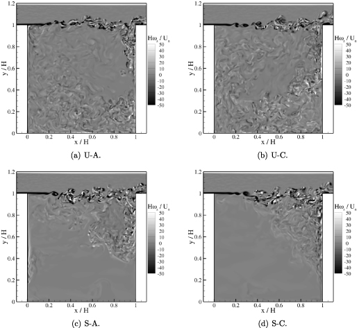
Figure 6. Contour map of normalised instantaneous spanwise vorticity within the cavity. Visualisations captured at an arbitrary time instant.
Download figure:
Standard image High-resolution imageIn all four simulations shown here, a vortex sheet is present immediately downstream of the leeward edge of the cavity. The vortex sheet rolls up into discrete K-H vortices, which then undergo pairing interactions that increase the thickness of the layer. At some distance downstream of the cavity edge, a pairing interaction results in the appearance of small scales in the shear layer, signifying the transition to turbulence. Qualitative changes in the evolution of the shear layer, dependent on the heating or cooling of the cavity walls, can be inferred from figure 6. For U-A, the heating of the leeward wall immediately below the separating shear layer results in a rapid generation of turbulence, and the shear layer appears to arch over the top of the cavity. In U-C, the shear layer evolution is similar to the neutral case (McMullan 2022), with the transition occurring at approximately mid-width of the cavity. Cooling of a cavity wall in S-A and S-C produces a qualitatively similar flow distribution — laminar K-H vortices undergo a rapid transition to turbulence at  , owing to the rapid acceleration of the flow produced by the primary cavity vortex inducing a highly turbulent flow field directly under the shear layer.
To provide a more quantitative assessment of the evolution of the cavity shear layer, profiles of the evolution of the streamwise r.m.s. velocity fluctuation along the top of the cavity,  , are shown in figure 7. For the neutral simulation, it has been shown that the evolution of the shear layer closely follows the prediction of vortex merging events (McMullan 2022) through the pairing parameter,
  , where the velocity ratio parameter
  , and θ is the momentum thickness of the separating boundary layer (Huang and Ho 1990). The shoulder in the profile at
  corresponds to a pairing parameter value of
  , indicating that the first generation of pairing interactions between K-H vortices occurs here. At
  there is a peak in the profile where the second generation of vortex amalgamation interactions occurs on average, such that
  , which precipitates the transition to turbulence in the cavity shear layer. As can be seen in figure 7, thermal stratification has a clear effect on the evolution of the cavity shear layer. For unstable stratification, heating of the leeward wall in U-A and U-All causes a more rapid evolution of the shear layer when compared to the neutral case. Heating the bottom wall also promotes an earlier transition to turbulence in the shear layer. The more rapid evolution of the shear layer in these simulations is linked to the enhanced fluctuations present near the leeward wall at the top of the cavity; buoyant fluid transported up the leeward wall towards the initial region of the cavity shear layer will induce fluctuations within the fluid, which will destabilise the vortex sheet immediately downstream of the cavity edge. The destabilisation of the shear layer will then promote its rapid evolution towards a fully turbulent state. Simulation U-C displays a shear layer evolution which is broadly similar to that of the neutral case.

Figure 7. Normalised streamwise velocity fluctuation profiles along the upper edge of the cavity,  .
.
Download figure:
Standard image High-resolution imageIn the stably stratified simulations, the evolution of the shear layer is markedly altered when compared to the neutral case. The lack of an obvious shoulder in the profiles demonstrates that the first generation of pairing events between K-H vortices precipitates the transition to turbulence in the cavity shear layer. The shifting of the recirculation vortex within the cavity results in a highly turbulent flow immediately underneath the shear layer, at the approximate location where the first pairing interaction takes place. The turbulent motions are of sufficient strength to trigger the transition to turbulence with the first pairing of K-H vortices. The above analysis demonstrates that, for cavity flows in which thermal stratification effects are important, the pairing parameter is no longer a valid representation of the vortex events which occur within the cavity shear layer.
Normalised mean temperature profiles recorded at  are shown in figure 8. The floor temperature is
  , and the normalising parameter is the absolute difference between the reference value and the temperature of a heated (or cooled) wall, i.e.
  . Heating of the leeward wall in U-A leads to only a minor increase in fluid temperature at the three measurement stations shown in figures 8(a)–(c). The updraft velocity induced by buoyancy has the same directional sense as the circulating fluid motion near the leeward wall, so high-temperature fluid is rapidly convected towards the cavity shear layer, where it mixes with ambient fluid. In U-B and U-C, the heating of the respective walls leads to more noticeable increase in fluid temperature in the cavity, and for U-All there is a marked increase in the mean fluid temperature. The influence of the vortex at the base of the cavity near the windward wall in simulations U-C and U-All is evident in the mean temperature profiles at
  , as shown in figure 8(c).

Figure 8. Normalised mean temperature profiles extracted from the simulations.
Download figure:
Standard image High-resolution imageThe mean temperature profiles in the stably stratified simulations show, with the exception of S-B, that the stagnant fluid present within the lower portion of the cavity attains a temperature close to that of the cooled surface. In S-All, the temperature of the fluid in almost the entire bottom half of the cavity is cooled. The shifting of the primary vortex towards the upper windward quadrant of the cavity limits the exchange of high-temperature ambient fluid from the freestream with the cooled fluid to a much smaller region in the cavity, as can be noted by the inflections in the temperature profiles. In S-B, where the primary vortex occupies the majority of the cavity, the recirculation of the vortex produces a relatively thin boundary layer of cooled fluid next to the cavity floor, with fluid of a near-ambient temperature elsewhere in the cavity.
The results presented above show that the flow within the cavity is altered by the heating, or cooling, of cavity walls. Unstable stratification through wall heating produces a strengthening of the cavity vortex, with a more rapid evolution of the cavity shear layer. Heating of the windward wall of the cavity produces a strong secondary vortex at the base of the windward wall, which is caused by the updraft associated with the effects of buoyancy on the fluid heated by the windward wall. The observations reported here are entirely consistent with both experiments (Allegrini et al 2013), and numerical simulations (Park et al 2012), of unstably stratified cavity flows above the critical Reynolds number.
Cooling of cavity walls to produce stably stratified flow results in a marked alteration of the flow-field. Cooling of the cavity floor leads to a flow-field which is qualitatively similar to the neutral case, whereas in all other configurations the primary vortex is pushed towards the windward wall and upwards towards the top of the cavity, resulting in a large region of stagnant fluid within the cavity. The evolution of the shear layer is delayed by stable stratification, and the proximity of the primary vortex alters the number of vortex amalgamations required for the transition to turbulence in the shear layer to occur.
In the next section, the effect of the changes to the flow-field on the dispersion of a contaminant will be assessed.
5. Tracer gas dispersion
Instantaneous normalised tracer gas concentration contour maps are shown in figure 9 for selected simulations. The images presented in figure 9 correspond to the same time instant at which the spanwise vorticity contour maps were obtained in figure 6. In U-A the tracer gas released at the line source (from the centre of the cavity floor) is transported towards the leeward wall, and then upwards along the leeward wall, by the rotation of the cavity vortex. The heating of the fluid next to the leeward wall enhances the updraft, and causes rapid entrainment of the tracer gas into the cavity shear layer, where it mixes with freestream fluid. The shear layer impinges on the windward wall of the cavity — some of the tracer gas propagates towards the outflow boundary, whilst the remainder re-enters the cavity. In addition, some tracer gas is recirculated within the cavity. The appearance of the large secondary vortex in U-C, observed in the mean streamlines of figure 2(d), alters the dispersion of the tracer gas within the cavity. The emitted gas is transported to the leeward wall and upwards towards the shear layer by the primary vortex, and entrained into the layer in a similar manner as that described for U-A. At the windward wall, however, a proportion of the fluid re-entering the cavity is diverted towards the cavity centre by the secondary vortex. Some of the tracer gas is entrained into the secondary vortex, where the buoyant motions induced by the heated windward wall cause it to recirculate in the corner of windward wall and the cavity floor.
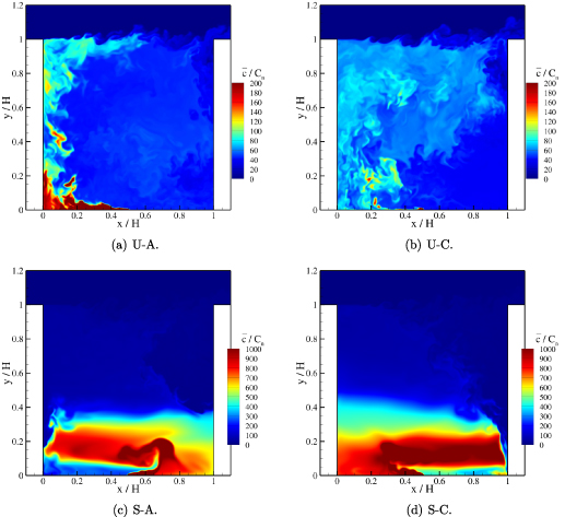
Figure 9. Contour map of normalised instantaneous tracer gas concentration within the cavity. Visualisations captured at the same time instant as the respective spanwise vorticity plot in figure 6. Note the changes in the contour levels between the stable, and unstable stratification cases.
Download figure:
Standard image High-resolution imageFigures 9(c) and (d) show the tracer gas concentration maps in S-A and S-C respectively. Note that the contour levels for the stable stratification simulations in figures 9(c) and (d) have increased by a factor of five, when compared to the unstable stratification simulations shown in figures 9(a) and (b). The downdraft produced by the cooling of the leeward wall in S-A is noticeable by the low values of tracer gas concentration found on both the leeward wall, and the leeward side of the cavity floor shown in figure 9(c). Similar penetration of low concentration fluid on the windward wall, and the windward section of the cavity floor is observed in S-C (figure 9(d)), as a result of cooling the windward wall. As noted above, both of these simulations contain a region of largely stagnant fluid in the lower half of the cavity. The line source jet is emitted into the stagnant fluid, producing a large excess of tracer gas at the cavity base. The fluid reaching the shear layer at the top of the cavity contains relatively low tracer gas concentration, hence it can be surmised that substantially less contaminant is removed from the cavity in these simulations. For S-B (not shown here), the tracer gas concentration map bears closer resemblance to the neutral case (McMullan 2022), owing to the relatively low displacement of the recirculation vortex with respect to that present at isothermal conditions.
Normalised mean concentration profiles for the unstable stratification simulations are shown in figures 10(a)–(c), along with the neutral experiment (Kikumoto and Ooka 2018) and simulation (McMullan 2022) data. At  simulations U-B, U-C, and U-All show a reduction in the mean tracer gas concentration, when compared with the neutral case. The reduction is a result of the enhanced circulation velocity of the primary cavity vortex, as noted in figures 2(c), (d) and (e), which decreases the residence time of the fluid in the cavity. The concentration profile for U-A is close to the neutral data. At
  , U-C predicts a general increase in the mean concentration, particularly near both the cavity base, and its upper quarter. The other profiles are close to the neutral data. Towards the windward wall, at
  , U-A, U-B and U-All yield an increase in the mean concentration in the upper half of the cavity when compared to the isothermal case, whilst an excess of tracer gas is found towards the cavity floor in U-C. The r.m.s. concentration fluctuations are shown in figures 10(d)–(f). Heating of the leeward wall has little effect on the concentration fluctuations in the cavity at
  , but enhanced fluctuation levels are present in the shear layer. All other simulations show a reduction in the r.m.s. concentration fluctuations at this location. At
  , U-C shows a substantial increase in the magnitude of the concentration fluctuations, owing to the presence of the large secondary vortex at the base of the cavity. The effect of this vortex on the concentration fluctuations can also be observed in the bottom half of the cavity at
  . The reduction of mean contaminant concentration in U-B is in agreement with other numerical predictions of cavity flows with ground heating (Li et al
2010). Furthermore, the results for U-B also qualitatively capture trends observed in experimental data of Uehara et al (2000), as shown in figure 10.
. The reduction of mean contaminant concentration in U-B is in agreement with other numerical predictions of cavity flows with ground heating (Li et al
2010). Furthermore, the results for U-B also qualitatively capture trends observed in experimental data of Uehara et al (2000), as shown in figure 10.

Figure 10. Concentration statistics obtained at various streamwise locations in the unstably stratified simulations. Case N, and experimental data, recorded at isothermal conditions.
Download figure:
Standard image High-resolution imageThe stagnant fluid present in the cavity in simulations S-A, S-C, and S-All, has a dramatic effect on the mean concentration profiles, as shown in figures 11(a)–(c). At  , the peak value of concentration increases by a factor of 2.6 in S-A, a factor of 4.0 in S-C, and a factor of 5.5 in S-All, when compared to the neutral data. Similarly at
  , the peak concentration increases by an order of magnitude over the neutral values in these three cases. Owing to the large values of the mean concentration, the associated r.m.s. fluctuations, shown in figures 11(d)–(f), are also large in the region of the stagnant fluid. The primary vortex occupies the majority of the cavity in simulation S-B, hence the tracer gas is transported around the cavity in a manner similar to that of the neutral case. There are substantially higher values of the mean concentration, and the r.m.s. fluctuation, near the floor of the cavity at
  in S-B — this is a result of the flapping of the tracer gas jet caused by the reduced circulation at the cavity base. The magnitude of increase in the mean contaminant in the stably stratified simulations presented here has also been observed in other simulations of cavity flows with ground cooling (Li et al
2016).
in S-B — this is a result of the flapping of the tracer gas jet caused by the reduced circulation at the cavity base. The magnitude of increase in the mean contaminant in the stably stratified simulations presented here has also been observed in other simulations of cavity flows with ground cooling (Li et al
2016).
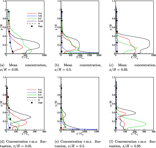
Figure 11. Concentration statistics obtained at various streamwise locations in the stably stratified simulations. Case N, and experimental data, recorded at isothermal conditions.
Download figure:
Standard image High-resolution imageThe mean mass of tracer gas in the cavity can be obtained through the evaluation of  . Table 4 outlines the mean tracer gas mass in the entire cavity at
  , and the mean mass contained within the lower 25% of the cavity. The ratio of mass in both the entire cavity and the bottom 25% of the cavity with respect to that present in case N is also provided. The mean mass within the cavity does not vary substantially between the neutral case, and all of the unstably stratified configurations, with the largest difference of 7% noted in U-B. Similarly, the lower quarter of the cavity contains approximately one-third of the total mass of tracer gas within the entire cavity for the neutral, and unstable stratification cases. For the stably stratified cases, simulation S-B shows an increase of 35% in the total tracer gas mass present in the cavity compared to the neutral data, and 53.6% of the contaminant is found in the lower quarter of the cavity. The mass of contaminant in the cavity S-A, S-C, and S-All increases by a factor of 3.296, 4.069, and 5.218 respectively over the neutral case. Along with the substantial increase in the total mass of contaminant, almost 75% of the total mass is found in the bottom quarter of the cavity. That cases S-A, S-C, and S-All display this dramatic increase in tracer gas mass in the cavity is significant, as all three cases show that the normal circulation of fluid within the cavity is disrupted by the primary vortex shifting to the upper quadrant of the cavity.
Table 4. Mean mass of tracer gas within the cavity in each simulation, along with the ratio compared to that of case N. Both the full cavity, and the bottom 25% of the cavity, are considered. Concentration mass is dimensionless.
| Case | Full cavity | Factor of N (full) | Bottom 25% of cavity | Factor of N (25%) |
|---|---|---|---|---|
| N | 65.2 | 1 | 23.4 | 1 |
| U-A | 64.6 | 0.991 | 23.2 | 0.991 |
| U-B | 60.6 | 0.929 | 19.4 | 0.829 |
| U-C | 62.0 | 0.951 | 19.9 | 0.850 |
| U-All | 61.1 | 0.937 | 19.6 | 0.838 |
| S-A | 214.9 | 3.296 | 162.9 | 6.962 |
| S-B | 88.3 | 1.354 | 47.4 | 2.026 |
| S-C | 265.3 | 4.069 | 188.2 | 8.043 |
| S-All | 340.2 | 5.218 | 248.1 | 10.603 |
The normalised vertical concentration fluxes,  , are shown in figure 12 for the neutral simulation, and cases where the windward wall, or the leeward wall, are heated or cooled respectively. The neutral case shows strong vertical concentration flux in the region of the shear layer where the first vortex pairing interaction takes place, and also in the region where the tracer gas jet is transported from the cavity floor by the action of the primary vortex. In U-A, the enhanced circulation velocity of the primary vortex reduces the magnitude of the vertical concentration flux in the tracer gas jet, and a region of enhanced vertical concentration flux is apparent near the heated leeward wall. The region of strong vertical flux near the windward wall is reduced, in comparison with the neutral case. The magnitude of the flux is diminished within the cavity shear layer, owing to the change in its evolution described above. For U-C, there is a strong vertical concentration flux where the tracer jet is emitted, owing to the presence of the secondary vortex in the lower windward wall corner. Similarly there is a strong flux at mid-height of the windward wall, near the stagnation point between the primary and secondary cavity vortices. The flux within the shear layer is altered, consistent with the delayed evolution of the layer noted in figure 7(a). Case S-A shows that the shear layer contains only very weak vertical concentration fluxes, given the relative absence of the tracer gas near the top of the cavity. Strong fluxes are observed at the tracer gas line source, where the jet issues into stagnant fluid, and at the lower portion of the leeward wall, where the downdraft of cooled fluid results in the complex local recirculation pattern observed in figure 2(f). A region of elevated flux resides at the interface between the primary cavity vortex and the stagnant fluid in the cavity, where significant quantities of tracer gas are entrained into the primary vortex. The entrainment process consequently produces a large region of negative flux in the central region of the cavity. In S-C, cooling of the windward wall produces extremely high magnitude vertical concentration fluxes at the lower corner of the windward wall, and at the tracer gas jet which issues into stagnant air. Relatively low fluxes are observed in the cavity shear layer in S-C, as relatively low quantities of the tracer gas reach the upper leeward quadrant of the cavity.

Figure 12. Contour maps of turbulent vertical concentration flux,  , recorded at mid-span of the domain,
  .
.
Download figure:
Standard image High-resolution imageConcentration PDFs are shown in figure 13, from three regions of interest in the cavity; at mid-height of the leeward wall,  (0.05, 0.5), at the centre of the cavity in the vicinity of the shear layer, (
 (0.5, 0.95), and at mid-height of the windward wall, (
 (0.95, 0.5).

Figure 13. Tracer gas concentration probability density functions, recorded at selected measurement points in the cavity. Note the changes in axes extents between the sub-figures.
Download figure:
Standard image High-resolution image
In the unstable stratification simulations, the PDF at  (0.05, 0.5) shows that the most probable concentration found in U-A, U-B, and U-All, is close to that observed in the neutral data. It is interesting to note that the larger peak in the most probable concentration also results in a reduction of the range of observed concentration values, and that higher concentration values are less likely to be observed when compared to the neutral data. The most probable value of tracer gas concentration at this location in case U-C is approximately 70% higher than the other simulations, but the much narrower range of observed concentrations results in a mean concentration at
  (0.05, 0.5) that is lower than the other cases. Given that the primary vortex location relative to the cavity shear layer is only weakly affected in the unstably stratified simulations, the PDFs observed in all cases at (
 (0.5, 0.95) are similar to that recorded in the neutral case. At (
 (0.95, 0.5), the influence of the secondary vortex on the PDF in U-C can clearly be observed, whilst all other cases show a shift in the range of recorded concentrations to higher values.
For the stably stratified cases, the concentration PDFs are widely different to the neutral data for all three measurement stations. In S-A, S-C, and S-All, significantly higher values of tracer gas concentration are found near to the leeward wall at  (0.05, 0.5), whilst markedly lower values are observed in both the region of the cavity shear layer,
  (0.95, 0.5), and at the mid-point of the windward wall, (
 (0.5, 0.95). The disruption to the circulation of fluid within the cavity in these three simulations leads to a build-up of high values of tracer gas concentration near the floor, and a resultant absence of the contaminant in the cavity shear layer. Given that the cavity shear layer contains only small amounts of tracer gas, the fluid which re-enters the cavity at the windward wall is largely composed of freestream fluid. It is only case S-B, where the primary cavity vortex remains largely near the centre of the cavity, that the distribution of the contaminant within the cavity bears any resemblance to the neutral data.
6. Conclusions
Thermal stratification has been found to (heavily) influence the transportation of tracer gas around the cavity as well as its removal by the cavity shear layer. Unstable stratification tends to increase the strength of the primary cavity vortex, whilst accelerating the evolution of the cavity shear layer thus promoting the entrainment and mixing of the tracer gas with the freestream fluid. This enhances the removal of tracer gas from the cavity although a portion of the contaminant gas remains entrapped within the cavity due to the primary recirculation. In contrast, in stable stratification the evolution of the shear layer is delayed and the number of vortex amalgamations required for transition to turbulence in the shear layer is altered due to the proximity of the primary vortex to the shear layer. These conditions as well as the fact that the primary vortex is shifted upwards towards the windward wall, cause the flow in the bottom part of the cavity to remain stagnant, as reflected by the stronger concentration of tracer gas in this region. Consequently, stable stratification results in poorer tracer gas transportation and removal around the cavity. The results presented in this paper show that unstable stratification enhances the pollutant dispersion and removal in the urban environment when compared to stable stratification.
Acknowledgments
This research was performed on ALICE2, the University of Leicester High Performance Computing Service. The research was supported through a Royal Academy of Engineering/Leverhulme Trust Research Fellowship, Grant Number LTRF1920 16 38.