


Abstract
We have examined the effects caused on the motion and sedimentation of a free falling solid particle by the hydrodynamic forces acting on the particle's surface arising when particle is close to wall. Drag and lift coefficients for a settling particle inside a narrow domain are calculated. An Eulerian mesh is adopted for computing the motion of free moving solid particles through the domain. The combined particle and fluid mixture is treated with a fictitious boundary method approach. To avoid particle-wall collisions, an approach proposed by Singh, Glowinsk and coauthors is used to handle such interactions. The particulate flow is computed using multigrid finite element solver FEATFLOW (Finite element analysis tool for flow problems). Numerical experiments are performed by decreasing domain widths for a single falling particle. The size and density of the particle is varied to inspect the particle paths. The behavior of the particle and its interaction with wall while it is moving inside constricted domains is analyzed. Results for the drag and lift forces on the surface of particle are presented and compared with the reference values.
Export citation and abstract BibTeX RIS
Recommended by Professor Hyung Jin Sung
1. Introduction
Particulate flows or motion of solid particles in fluids have a wide range of industrial applications, such as fluidized suspensions, depositions formed due to flowing suspension of particle, lubricated transport, medical related industry, sedimentation, hydraulic fracturing of reservoirs, slurry flow, paper pulp, food products etc. These types of flows are common in many natural processes such as dust particles in air, mud flow, sand storms, ocean current interaction with offshore structures, lava flow and sedimentation in estuary etc. Particulate flows have been a subject of great importance with research contributions coming from the field of biology, chemistry, physics, engineering and mathematics. Study of soft solids has practical applications in the the field of bio-medicine and involve the study of hemodynamics and suspended blood cells (Fogelson and Guy 2004). Particulate flows are quite complex and hard to simulate numerically, because frequent generation and deformation of computational grid is required in many cases when the particle boundaries are complex and moving with time. The problem becomes more complex in the case with large number of particles due to fluid particle interaction as well as due to particle-particle and particle-wall collisions.
Several techniques to simulate particulate flows numerically have been evolved over the years such as discrete element models (Glowinski et al 1999, Patankar et al 2000, Singh et al 2003), penalty based methods (Glowinski et al 1999, Sokolov et al 2015), population balance models (Glowinski et al 1999), level-set methods (Glowinski et al 1999), the cut-cell finite volume approach (Clarke et al 1986), and distributed Lagrange multiplier (DLM) fictitious domain methods (Glowinski et al 1999, Walayat et al 2018a, 2018b). The hydrodynamic forces acting on the particles are obtained by resolving the flow field around each particle. These methods are mainly categorized into two groups, Eulerian approach and the Lagrangian approach. In the first approach a fixed mesh is used which covers the domain occupied by the fluid and solid particles move independently inside the domain. DLM/fictitious domain method proposed by Glowinski et al (1999), Patankar et al (2000), Singh et al (2003)is one of the famous examples of this approach. The second approach is based on following the moving particle boundaries by the mesh nodes. This approach is usually called arbitrary Lagrangian Eulerian which is extensively used by Glowinski et al (1999), Patankar et al (2000), Singh et al (2003), Maury Hirt et al (1974), Hughes et al (1981, 1996), Nitikitpaiboon and Bathe (1993), Hu et al (2001), Fauci and McDonald (1995), and deforming-spatial-domain/stabilized-space-time approach of Tezduyar et al (1992). A big advantage of Eulerian technique over the Lagrangian technique is that the computational mesh is not changed with the particle motion, thus saves CPU cost per time step but the resulting accuracy is some times not as high as for the Lagrangian case. Therefore in these methods, the overall objective is to deal with the moving boundaries in the fluid successfully, improve the accuracy of the numerical approximation and reduce the computational cost. These methods have been widely used to study fluid-particle interaction (FPI) problems (Johnson and Tezduyar 1997, 2001), parachute modeling (Stein et al 2001), moving hyperelastic particles (Gao and Hu 2009), sperm motility near boundaries (Fauci and McDonald 1995), modeling rigid particles (Usman et al 2018, Jabeen et al 2019, Walayat et al 2019, 2020), modeling flexible bodies (Zhao et al 2008), red blood cell (Gong et al 2009) and modeling blood flow in heart (Watanabe et al 2004). Relatively less popular methods to deal fluid-particle methods are mesh free methods such as the reproducing kernel particle method and smoothed particle hydrodynamics (Oñate et al 2008).
Investigation of particle interaction with wall and its impact on the overall behavior of the fluid-particle system is of great importance and has been a subject of research. Chein and Liao (2005) analyzed particle-wall interaction during particle free fall. They presented more understanding of particle deposition onto collector surfaces using Lagrangian method and studied how the particle approach the region near the wall and the mechanism that causes the particles to deposit onto the wall.
To prevent particle collisions with wall, a collision model is required to avoid particle overlap with wall. Such overlapping occurs due to numerical errors faced during simulations but are not possible physically. Different collision models have been proposed in literature to handle this problem numerically. Some of the collision models are repulsive force models (Glowinski et al 1999), lubrication collision models (Glowinski et al 1999), conservation collision models (conservation of linear momentum and kinetic energy) (Glowinski et al 1999), stochastic collision models (physical properties of the particle) (Glowinski et al 1999), semi-experiential collision models, etc. For solving this problem, Glowinski et al (1999), Patankar et al (2000), Singh et al (2003)have presented repulsive force models to prevent particles from overlapping. Their idea was to allow hydrodynamic lubrication forces to act up to the full tolerance of the mesh and allow the particles to pack naturally in equilibrium.
The present study contributes in numerical inspection for the drag and lift forces affecting a single falling circular particle. A detailed examination of the hydrodynamic forces arising when the particle is near to the wall of the channel is carried out and the behavior of the particle and its motion is discussed. The coupled solution of incompressible fluid flow and settling solid particle is achieved using a direct simulation technique called fictitious boundary method (FBM) (Turek et al 2003). The Eulerian based background mesh is adopted which is independent of particle number, shape and size.
2. Mathematical modeling
Consider fluid flow along with a solid particle with mass Mr
and density of particle ρr
. The fluid has density ρw
and ν represents the fluid viscosity. The fluid occupies the domain  and the domain of particle is represented by
  .
.  represents boundary of the particle. Hence, the total domain is given by
2.1. Incompressible fluid flow and the independent particle motion
The incompressible fluid motion in the domain  is governed by the Navier–Stokes equations (John 2002, Turek et al
2006, Wendt 2009)
is governed by the Navier–Stokes equations (John 2002, Turek et al
2006, Wendt 2009)

where the total stress tensor σ in the fluid phase is defined as,

Here, the velocity of fluid is u , p is the pressure, coefficient of viscosity is µw and I stands for the identity tensor.
The translational and rotational motion of the freely moving rigid particle in fluid is due to the hydrodynamic forces acting on the surface of particle, collision forces arising between approaching particle and outer wall and gravitational acceleration. The Newton–Euler equations in this case, take the form

The translational velocity of the particle is
U
r
and ωr
is the angular velocity of the particle, Mr
is the particle mass and we can find  , where Mw
is the mass occupied by the fluid having the same volume as the volume of Mr
. Drag and lift forces acting on the surface of particle are represented by
F
r
,
, where Mw
is the mass occupied by the fluid having the same volume as the volume of Mr
. Drag and lift forces acting on the surface of particle are represented by
F
r
,  are the collision forces acting on the particle, the moment of inertia tensor is
I
r
and the resultant torque acting about the center of mass of the particle is
T
r
.
g
denotes the gravitational acceleration.
are the collision forces acting on the particle, the moment of inertia tensor is
I
r
and the resultant torque acting about the center of mass of the particle is
T
r
.
g
denotes the gravitational acceleration.
The position X r of the center of mass of the particle and its angle θr can be obtained after integrating the following kinematic equations (Wan et al 2004, Wan and Turek 2006),

2.2. Drag and lift hydrodynamic forces and torque
The drag and lift forces F r and the torque T r acting on the mass center of the particle can be obtained by Kim and Karrila (1991)

where the unit vector
n
acts normal to the boundary  of the particle. Once the drag force is calculated, the drag and lift coefficients can be found using

where U and D is the characteristic velocity and length respectively.
2.3. Coupling particle and fluid phase with FBM
The fluid and particle mechanism is coupled together by applying the no-slip boundary conditions at the interface between the fluid and particle's surface  , where the velocity at the surface of the particle
  is given by,

The FBM operates over a multigrid finite element method by incorporating the boundary conditions in the fluid domain obtained from the velocity of the particle domain. The additional constraints arising due to the moving boundary of the particle at the particle-fluid interface are included in the Navier–Stokes equations, by extending the fluid domain with the combined fluid and particle domain, which takes the form,
2.4. Treatment of particle-wall collisions
We will use a collision model for the evaluation of particle-wall collision forces  presented by Patankar et al (2000).
where  is the coordinate of the center of mass of the nearest imaginary particle
  imagined on the boundary wall with respect to the particle.
  is the distance between the center of the imaginary particle
  and the mass center of particle. ρ is the minimum distance to activate the force of repulsion between particle and cylinder and is taken one mesh element apart in our case because a very fine mesh is used having size approximately 10−2 . εr
and
and the mass center of particle. ρ is the minimum distance to activate the force of repulsion between particle and cylinder and is taken one mesh element apart in our case because a very fine mesh is used having size approximately 10−2 . εr
and  are small positive stiffness parameters for particle-wall collisions and their values are taken in between 10−5 and 10−6 in the calculation so that discontinuity or singularity is avoided.
3. Fractional-step-θ scheme
A strongly stable fractional-step-θ time-stepping scheme is applied for time discretization. For the case of rough initial or boundary data its smoothing property is essential. It also has little numerical dissipation that is critical for the calculation of non-enforced temporal oscillations. For a detailed description, readers are referred to articles (Turek 1996, 1997). Initially, the semi-discretization of equation (8) is performed by using the fractional-step-θ scheme provided that un
and time step  and then solve for
  and
and  . The fractional-step-θ scheme splits one macro-time step
  into three consecutive sub steps with
where  ,
,  ,
,  ,
,  , N(v)u is a compact form for the diffusive and convective part as follows:

Hence, by using equation (10) in each time step, it is required to solve non-linear problems of the following type:

Finally, an explicit expression for equation (8) (c) is used as follows:

4. Discrete projection method
In order to solve discrete non-linear problems after space and time discretization, some steps need to be taken into account such as treatment of incompressibility and non-linearity, convergence criteria for the overall outer iteration, convergence control, number of splitting steps and embedding into multi-grid. Initially, the coupled problem is split to obtain the definite problem in u (Burgers equations) as well as in p (pressure Poisson problems). Afterwards, non-linear problems in velocity u are tackled through the appropriate non-linear iteration or linearization technique, and a multi-grid solver is used to solve Poisson-like problems.
5. Numerical investigations
In this section, we will present results of the numerical experiments performed using CFD code FEATFLOW (Turek 1998). We will analyze and observe the kinetics of a single particle settling due to gravity inside a channel when it is passing near the wall of the domain. First, the numerical results of a single particle in an infinite vertical channel and the hydrodynamic forces acting on the particle as it falls due to gravity are presented. Then, the results for a particle passing nearby the wall of the domain are discussed using different cases in such a way that the mesh width is reduced gradually. Moreover, various cases for different sizes and densities of the particle are considered in the study.
5.1. Drag and lift forces acting on the surface of a settling particle inside a vertical channel
Numerical experiments are performed to analyze and observe a solid particle freely falling inside a fluid channel under the action of gravity. The computational domain consists of a vertical channel having length 8.0 and width 2.0 containing fixed equidistant mesh elements. The particle is a rigid 2D circular solid with three distinct radii R = 0.115, R = 0.125, R = 0.135 and two different densities  ,
,  and is falling down due to gravitational acceleration g = 981 in an incompressible fluid. The density of fluid is
  and viscosity is
  . We have used the value of Reynolds number Re = 100. Assume that the particle and the fluid are initially at rest. The simulations are carried out on four different levels of mesh refinement. i.e. Level-3, Level-4, Level-5 and Level-6 where number of elements on coarse mesh are 196. The well known finite element pair Q2P1 has been adopted for the space discretization. In the reference calculation, Level-6 of the mesh is used.
Figure 1 shows a single falling rigid particle inside a vertical channel at different times. The particle tumbles, wobbles and forms a zigzag path during its course.

Figure 1. Snapshots of a single particle settling under gravity.
Download figure:
Standard image High-resolution imageThe reference level-6 shown in figure 2 (left) displays the drag and figure 2 (right) displays the lift coefficient values with respect to time for later comparison and analysis with lower refinement mesh levels.
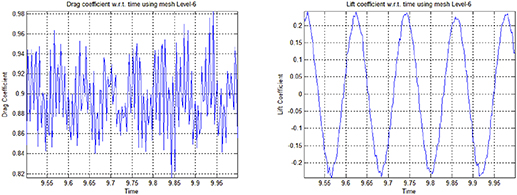
Figure 2. Drag Cd and Lift Cl coefficients w.r.t. time using mesh level-6.
Download figure:
Standard image High-resolution imageFigures 3–5 show drag and lift coefficients with respect to time. Plots on the left show drag coefficients and pots on the right show lift coefficients with respect to time on different levels of mesh refinement for a 2D circular particle falling due to gravity inside a channel. We have selected the time interval from t = 9.5 to t = 10 for these graphs when the particle attains the terminal velocity. The graphs clearly show that by increasing the mesh refinement level the drag coefficient shows more periodic oscillations with respect to the time, where as the oscillations in the lift coefficients decreases by increasing the mesh refinement level with respect to the time. We can see that the drag and lift coefficients shows better periodic behavior as the mesh refinement level increases.
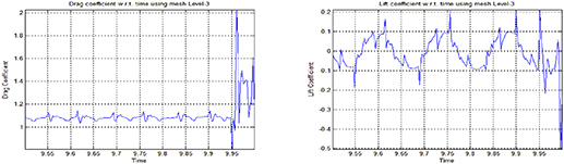
Figure 3. Drag Cd and Lift Cl coefficients w.r.t. time using mesh level-3.
Download figure:
Standard image High-resolution image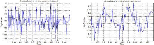
Figure 4. Drag Cd and Lift Cl coefficients in time using mesh level-4.
Download figure:
Standard image High-resolution image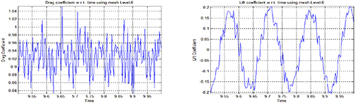
Figure 5. Drag Cd and Lift Cl coefficients w.r.t. time using mesh level-5.
Download figure:
Standard image High-resolution imageTable 1 presents the maximum and minimum values of drag and lift coefficients on different levels of mesh refinement, for a 2D circular particle falling inside a channel, due to gravity. Table 1 shows that the minimum value of drag coefficient gradually increases and the maximum value gradually decreases while converging toward the reference values. Similarly the minimum value of lift coefficient gradually increases and the maximum value gradually decreases while converging toward the reference values. A slight difference in drag and lift values at level-5 and level-6 can be observed but mesh refinement level-5 can still be used to simulate the falling particle.
Table 1. Drag Cd and Lift Cl coefficients for a circular ball falling inside a channel.
| Drag coefficient Cd | Lift coefficient Cl | ||||
|---|---|---|---|---|---|
| LEVEL | NEL | Cd Min | Cd Max | Cl Min | Cl Max |
| 3 | 3136 | 0.6000 | 2.4119 | −0.5026 | 0.4390 |
| 4 | 12 544 | 0.7489 | 1.4525 | −0.3512 | 0.3110 |
| 5 | 50 176 | 0.8010 | 1.0635 | −0.2191 | 0.2253 |
| 6 | |||||

| 200 704 | 0.8152 | 0.9894 | −0.2489 | 0.2510 |
5.2. Behavior of falling particle inside a channel with different mesh sizes and varying positions
A free falling particle while interacting with a neighboring wall has been examined. The particle is moving inside a narrow channel having different widths. Numerical experiments have been performed by taking an infinite vertical channel with width 2.0 and height 8.0 (Mesh 1). In the second case, the mesh is chopped from both sides using lengths 0.2 and the width is reduced to 1.6 (Mesh 2).
A similar procedure is adopted and another mesh is obtained with width 1.2 by chopping the two sides (Mesh 3) and finally a very narrow mesh is obtained by chopping a length of 0.1 from both sides so that the new mesh has width 1.0 (Mesh 4). The meshes are chopped from both ends such that the center of each mesh is kept at x = 1.0 (see figure 6). An extensive study is conducted by considering three radii for the solid particle, R = 0.115, R = 0.125, R = 0.135 and two values for the density,  ,
,  , falling with gravitational acceleration g = 981 in an incompressible fluid having density
  and viscosity
  (see figure 7).
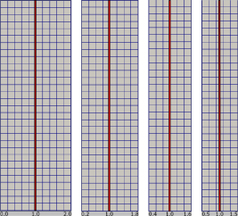
Figure 6. Mesh schematic level-3.
Download figure:
Standard image High-resolution image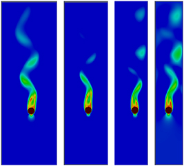
Figure 7. Snapshots of a single particle falling under gravity.
Download figure:
Standard image High-resolution imageParticle is released from a height y = 0.6. Four starting positions for the particle in x-direction are considered that is at x = 0.95 (far from the wall), x = 0.55, x = 0.35 and x = 0.15 (very near to wall) using Mesh 1. Three starting positions for the particle in x-direction are considered that is at x = 0.95 (far from the wall), x = 0.55 and x = 0.35 (very near to wall) using Mesh 2. Similarly, two starting positions for the particle in x-direction are considered that is at x = 0.95 (far from the wall) and x = 0.55 (very near to wall) using Mesh 3. Only one position x = 0.95 is chosen for Mesh 4.
Figure 8 left shows graphs for particle's x-positions with respect to time keeping four different starting positions and figure 8 right shows graphs for particle's x-positions with respect to time keeping four meshes of different widths. Figure 8 shows that the particle gets a push from the wall and moves away from the wall as it falls down. The more particle is close to the wall the more it is pushed away from the wall. Similarly, keeping the same starting position and using meshes of different widths, it has been observed that for a more narrower mesh the particle experiences more thrust from the wall.
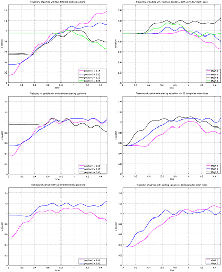
Figure 8. Trajectory of particles with different starting positions and different mesh sizes using ρ = 1.25,  .
.
Download figure:
Standard image High-resolution imageFigure 9 shows that by decreasing the radius of the particle, the particle experiences more thrust from the wall and moves more toward the right wall. On the other hand, figure 10 shows that by increasing the density of the particle, the particle shows less movement toward the right wall and impact of the hydrodynamic forces is reduced.

Figure 9. Trajectory of particles with different starting positions and different mesh sizes using ρ = 1.25,  .
.
Download figure:
Standard image High-resolution image
Figure 10. Trajectory of particles with different starting positions and different mesh sizes using ρ = 1.50,  .
.
Download figure:
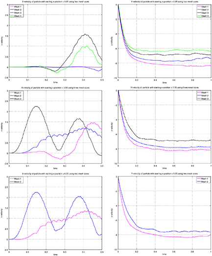
Standard image High-resolution imageFigure 11 left shows graphs for particle's x-velocity with respect to time and figure 11 right show graphs for the particle's y-velocity with respect to time. In all the graphs it is clear that the particle attains a terminal velocity in the y-direction after some instance during the fall. Figure 11 shows that particle attains more y-velocity for the same starting position of a particle if the channel is less narrower but on the other hand the particle attains less vertical velocity and falls slowly if the channel is very narrow. Hence the terminal velocity of the particle in case of a narrower channel is less than the terminal velocity in case of a wider channel.
Figure 11. Velocities of particles with different starting positions and different mesh sizes.
Download figure:
Standard image High-resolution image
Table 2 presents a comprehensive comparison of particle trajectories and velocities using meshes of different widths. It has been observed that the starting position of the particle contributes a major part in defining the course of the particle. If the particle is started from a position which is very near to the left wall then it gets more push from the wall and moves toward the right wall more quicker than if a particle is started a bit away from the left wall.
Table 2. Particle kinetics with different starting positions of settling particle in a channel having fixed width using ρ = 1.25,  .
.
| Channel 1 | |||||
|---|---|---|---|---|---|
| Starting x-position | Time at x = 1.0 | Speed at x = 1.0 | Maximum x-position | Time at max. x-position | Distance from right wall at max x shift |
| 0.15 | 0.834 | 0.081 | 1.427 | 1.767 | 0.573 |
| 0.35 | 0.873 | 0.318 | 1.207 | 1.623 | 0.793 |
| 0.55 | 0.975 | 0.399 | 1.009 | 1.014 | 0.991 |
| 0.95 | 0.885 | 1.725 | 1.009 | 0.918 | 0.991 |
| Channel 2 | |||||
| 0.35 | 0.597 | 0.075 | 1.070 | 2.553 | 0.730 |
| 0.55 | 0.675 | 0.210 | 1.070 | 1.272 | 0.730 |
| 0.95 | 0.609 | 0.576 | 1.070 | 2.349 | 0.730 |
| Channel 3 | |||||
| 0.55 | 0.420 | 0.069 | 1.104 | 0.867 | 0.496 |
| 0.95 | 0.375 | 0.330 | 1.270 | 1.917 | 0.330 |
| Channel 4 | |||||
| 0.95 | 0.423 | 0.354 | 1.152 | 0.687 | 0.348 |
The table 2 also presents the speed of the particle when it reaches at the center of the channel, that is at x = 1.0. It can bee seen that particle reaches the center of the channel quickly while consuming less time if it is started from a position near to the left wall. As we decrease the width of the channel, the speed of the particle increases and reaches the center in less time as compared to a channel which is wider as can be seen from results of Channel 1, Channel 2, Channel 3 and Channel 4.
Table 3 confirms that by decreasing the particle radius, the particle takes more x-shift and attains the maximum x-shift in lesser time as compared to a bigger particle. Table 4 shows that by increasing the density of the particle the x-shift toward the right wall is reduced but on the other hand the time to reach the maximum x-shift is further reduced.
Table 3. Particle kinetics with different starting positions of settling particle in a channel having fixed width using ρ = 1.25,  .
.
| Channel 1 | |||||
|---|---|---|---|---|---|
| Starting x-position | Time at x = 1.0 | Speed at x = 1.0 | Maximum x-position | Time at max. x-position | Distance from right wall at max x shift |
| 0.15 | 0.294 | 0.300 | 1.649 | 1.128 | 0.351 |
| 0.35 | 1.017 | 0.201 | 1.518 | 2.304 | 0.482 |
| 0.55 | 1.134 | 0.156 | 1.071 | 1.416 | 0.929 |
| 0.95 | 2.556 | 0.090 | 1.197 | 2.670 | 0.803 |
| Channel 2 | |||||
| 0.35 | 0.249 | 0.231 | 1.372 | 2.553 | 0.428 |
| 0.55 | 1.992 | 0.147 | 1.365 | 2.295 | 0.435 |
| 0.95 | 2.133 | 0.081 | 1.267 | 2.529 | 0.533 |
| Channel 3 | |||||
| 0.55 | 0.219 | 0.189 | 1.220 | 2.304 | 0.380 |
| 0.95 | 0.714 | 0.069 | 1.170 | 2.817 | 0.430 |
| Channel 4 | |||||
| 0.95 | 0.204 | 0.159 | 1.258 | 2.373 | 0.242 |
Table 4. Particle kinetics with different starting positions of settling particle in a channel having fixed width using ρ = 1.50,  .
.
| Channel 1 | |||||
|---|---|---|---|---|---|
| Starting x-position | Time at x = 1.0 | Speed at x = 1.0 | Maximum x-position | Time at max. x-position | Distance from right wall at max x shift |
| 0.15 | 0.213 | 0.195 | 1.325 | 0.663 | 0.675 |
| 0.35 | 0.381 | 0.141 | 1.099 | 0.516 | 0.901 |
| 0.55 | 0.438 | 0.111 | 1.180 | 3.000 | 0.820 |
| 0.95 | 0.477 | 0.051 | 1.180 | 3.000 | 0.820 |
| Channel 2 | |||||
| 0.35 | 0.192 | 0.168 | 1.221 | 0.384 | 0.579 |
| 0.55 | 0.330 | 0.102 | 1.151 | 0.543 | 0.649 |
| 0.95 | 0.411 | 0.048 | 1.124 | 0.621 | 0.676 |
| Channel 3 | |||||
| 0.55 | 0.174 | 0.135 | 1.147 | 0.309 | 0.453 |
| 0.95 | 0.285 | 0.042 | 1.218 | 0.765 | 0.382 |
| Channel 4 | |||||
| 0.95 | 0.162 | 0.111 | 1.187 | 0.462 | 0.313 |
6. Conclusion
In this work, we used FBM coupled with the Finite Element Method to simulate the experiments. The main focus of the study was to examine the behavior of immersed falling particle inside narrow domains and the effect of wall forces acting on the particle's surface. A novel analysis has been presented to examine the behavior of particle inside constricted domains and effect on the velocity of the falling particle has been discussed. It is concluded that the width of the channel, starting position, density and radius of the particle play an important role in defining the path and movement of the particle. The above factors and the FPIs result in an inconsistent hydrodynamic drag forces acting on the surface of the particle and cause vortex shedding and vortex formations of different sizes and shapes.
The computed results for a single falling particle inside computational domains of different widths showed different settling behavior of particle and a gradual change in particle velocities at different configurations for varying starting positions of particle. The results are computed on mesh refinement level-6. The analysis was carried out by taking four initial positions of the particle and has been tested with four vertical channels of different widths along with three particle radii and two different particle densities. The analysis includes trajectories of the particle, estimated shift of the particle toward the right wall of the domain, terminal velocities attained by the particle while settling down and the time taken to cross the center of the domain.
In future, it is desired to compare the numerical results while placing circular cylinders inside the channel at different positions and to observe the behavior of the particle while it crosses these hurdles. We also intend to investigate the results by changing the shape of the cylinders, such as square cylinders, and by increasing the number of cylinders.
Acknowledgment
This work was supported by the HEC National Research Program for Universities—NRPU 2020 [Grant No. 14038].