

Abstract
This paper assesses the prediction of inert tracer gas dispersion within a cavity of height (H) 1.0 m, and unity aspect ratio, using large Eddy simulation (LES). The flow Reynolds number was 67 000, based on the freestream velocity and cavity height. The flow upstream of the cavity was laminar, producing a cavity shear layer which underwent a transition to turbulence over the cavity. Three distinct meshes are used, with grid spacings of  (coarse),
  (intermediate), and
  (fine) respectively. The Smagorinsky, WALE, and Germano-Lilly subgrid-scale models are used on each grid to quantify the effects of subgrid-scale modelling on the simulated flow. Coarsening the grid led to small changes in the predicted velocity field, and to substantial over-prediction of the tracer gas concentration statistics. Quantitative metric analysis of the tracer gas statistics showed that the coarse grid simulations yielded results outside of acceptable tolerances, while the intermediate and fine grids produced acceptable output. Interrogation of the fluid dynamics present in each simulation showed that the evolution of the cavity shear layer is heavily influenced by the grid and subgrid scale model. On the coarse and intermediate grids the development of the shear layer is delayed, inhibiting the entrainment and mixing of the tracer gas into the shear layer, reducing the removal of the tracer gas from the cavity. On the fine grid, the shear layer developed more rapidly, resulting in enhanced removal of the tracer gas from the cavity. Concentration probability density functions showed that the fine grid simulations accurately predicted the range, and the most probable value, of the tracer gas concentration towards both walls of the cavity. The results presented in this paper show that the WALE and Germano-Lilly models may be advantageous over the standard Smagorinsky model for simulations of pollutant dispersion in the urban environment.
Export citation and abstract BibTeX RIS

Original content from this work may be used under the terms of the Creative Commons Attribution 4.0 license. Any further distribution of this work must maintain attribution to the author(s) and the title of the work, journal citation and DOI.
Recommended by Professor Hyung Jin Sung
1. Introduction
The dispersion of a contaminant within a cavity is a geometrically simple flow type, where the shear layer which develops over the top of the cavity acts to remove the contaminant from it. The shear layer typically contains turbulent vortex structures (Brown and Roshko 1974) which are responsible for the entrainment of the contaminant from the cavity, and mixing it with ambient freestream air (Konrad 1976, Koochesfahani and Dimotakis 1986, Karasso and Mungal 1996). Enhancement of contaminant removal from the cavity therefore requires an understanding of the evolution of the turbulent vortex structures, along with the mixing processes which occur within them.
Numerical simulation techniques are becoming an increasingly popular means to study the dispersion of contaminants within a cavity, due to the relevance of the flow configuration to vehicular pollutant dispersion within Urban Street Canyons (USCs). As over 50% over the global population live in urban areas (Department of Economic and Social Affairs, World urbanization prospects: 2014 Revision 2014), there is a clear need to both understand, and mitigate against, the effect of air pollution in urban environments (Burnett et al
2000, Cohen et al
2005). Conventional Reynolds-Averaged Navier–Stokes (RANS) methods, where all of the turbulent scales of motion in the flow are modelled, are unsuitable for the study of pollutant dispersion as the large-scale eddies responsible for the transport of pollutants in the cavity are not resolved, leading to inaccurate predictions (Salim et al
2011, Tominaga and Stathopoulos 2016). Direct numerical simulation (DNS), in contrast, solves all scales of motion explicitly and offers a complete description of the flow field. The computational expense required to undertake DNS limits this method to flows of low Reynolds number (Coceal et al
2007, Goulart et al
2018). It has been recognised that large Eddy simulation (LES) is an ideal numerical tool for the study of contaminant dispersion in a cavity, as the method has the capability to resolve the large scale structures which transport the contaminant in the flow at relatively low computational expense. In LES studies of pollutant dispersion in urban environments, the USC is typically represented as a cavity surrounded by solid walls (i.e. buildings), with spanwise periodic boundary conditions imposed. The base of the cavity can essentially be considered as a road, from which vehicular traffic pollutants are emitted through a source. Research has classified the flow regimes that can exist in a cavity, which depends on the aspect ratio of the cavity height, H, to the width between the buildings, W. Three regimes have been identified; skimming flow, for  0.7, wake interference flow for 0.3
  0.7, and isolated roughness flows for
  0.3 (Oke 1988). For skimming flow in a two-dimensional cavity, the wind flow perpendicular to the cavity will separate from the leeward wall at roof level, resulting in the formation of a shear layer. The shear layer impinges on the windward wall, and the transfer of momentum into the cavity establishes a large primary recirculation vortex within it. Pollutants emitted at ground level will circulate towards the leeward wall, and upward towards the shear layer, resulting in high levels of pollutant concentration near the leeward wall at pedestrian height. Once at roof level, the pollutant can be entrained into the shear layer and removed from the cavity through turbulent flux (Li et al
2015), but a proportion of the pollutant remains trapped within the cavity owing to the primary recirculation (Cheng et al
2008). The large-scale structures in the cavity shear layer play an important role in the transport of pollutants out of the cavity, as the dynamics of these structures govern the entrainment of fluid into the shear layer (Salizzoni et al
2009, Di Bernardino et al
2018). In addition to the shear layer, and the primary recirculation vortex, corner vortices will be present at the base of both the leeward wall, and the windward wall (Li et al
2021). Previous numerical research into the idealised USC have studied the effects of cavity aspect ratio (Assimakopoulos et al
2003, Liu et al
2005), reacting pollutants (Baker et al
2004, Kikumoto and Ooka 2012, Zhong et al
2017, Han et al
2018), and thermal stratification (Li et al
2010).
0.3 (Oke 1988). For skimming flow in a two-dimensional cavity, the wind flow perpendicular to the cavity will separate from the leeward wall at roof level, resulting in the formation of a shear layer. The shear layer impinges on the windward wall, and the transfer of momentum into the cavity establishes a large primary recirculation vortex within it. Pollutants emitted at ground level will circulate towards the leeward wall, and upward towards the shear layer, resulting in high levels of pollutant concentration near the leeward wall at pedestrian height. Once at roof level, the pollutant can be entrained into the shear layer and removed from the cavity through turbulent flux (Li et al
2015), but a proportion of the pollutant remains trapped within the cavity owing to the primary recirculation (Cheng et al
2008). The large-scale structures in the cavity shear layer play an important role in the transport of pollutants out of the cavity, as the dynamics of these structures govern the entrainment of fluid into the shear layer (Salizzoni et al
2009, Di Bernardino et al
2018). In addition to the shear layer, and the primary recirculation vortex, corner vortices will be present at the base of both the leeward wall, and the windward wall (Li et al
2021). Previous numerical research into the idealised USC have studied the effects of cavity aspect ratio (Assimakopoulos et al
2003, Liu et al
2005), reacting pollutants (Baker et al
2004, Kikumoto and Ooka 2012, Zhong et al
2017, Han et al
2018), and thermal stratification (Li et al
2010).
Effective use of LES requires particular attention to be paid to the grid resolution, and to the subgrid-scale model employed to close the governing equations. The resolution of the computational grid is a critical aspect of LES of contaminant dispersion in cavities, as it is important to resolve the vortex structures which transport the contaminant. In LES, scales of motion larger than the filter width (typically the cube root of the cell volume) are computed explicitly, and scales of motion smaller than the filter width are modelled using a subgrid-scale model. Computational resources have permitted grid spacings of  (Michioka et al
2011),
(Michioka et al
2011),  (Li et al
2010), and
(Li et al
2010), and  (Han et al
2018), in two-dimensional urban street canyons. More refined grids spacings of
(Han et al
2018), in two-dimensional urban street canyons. More refined grids spacings of  and
and  have been to simulate tracer gas dispersion in a simplified cavity, in order to provide a quantitative assessment of the grid resolution on both the mean concentration, and the concentration variance (Kikumoto and Ooka 2018). Many subgrid-scale models exist in the literature, which have been applied to shear layer simulations. For the spatially-developing shear layer originating from laminar conditions, it has been shown that the Smagorinsky model can delay the evolution of the mixing layer owing to artificially high subgrid viscosity in the laminar region (McMullan et al
2015, Huang et al
2021). The dynamic Smagorinsky model (Germano et al
1991, Lilly 1992) (also known as the Germano-Lilly model) corrects the deficiencies of the Smagorinsky model in mixing layer simulations through the dynamic computation of the model constant by a test-filtering process (Vreman et al
1997). It has also been shown, for plane turbulent mixing layers, that the WALE model (Nicoud and Ducros 1999) can also accurately capture the mixing layer development, and is largely insensitive to the choice of model constant (McMullan et al
2015). In USC/cavity simulations where shear flow plays a crucial role in the transport of pollutants from the cavity, however, the use of the Smagorinsky model remains widespread (Tominaga et al
2008, Cheng and Liu 2011, Tominaga and Stathopoulos 2011, Kikumoto and Ooka 2012, 2018).
have been to simulate tracer gas dispersion in a simplified cavity, in order to provide a quantitative assessment of the grid resolution on both the mean concentration, and the concentration variance (Kikumoto and Ooka 2018). Many subgrid-scale models exist in the literature, which have been applied to shear layer simulations. For the spatially-developing shear layer originating from laminar conditions, it has been shown that the Smagorinsky model can delay the evolution of the mixing layer owing to artificially high subgrid viscosity in the laminar region (McMullan et al
2015, Huang et al
2021). The dynamic Smagorinsky model (Germano et al
1991, Lilly 1992) (also known as the Germano-Lilly model) corrects the deficiencies of the Smagorinsky model in mixing layer simulations through the dynamic computation of the model constant by a test-filtering process (Vreman et al
1997). It has also been shown, for plane turbulent mixing layers, that the WALE model (Nicoud and Ducros 1999) can also accurately capture the mixing layer development, and is largely insensitive to the choice of model constant (McMullan et al
2015). In USC/cavity simulations where shear flow plays a crucial role in the transport of pollutants from the cavity, however, the use of the Smagorinsky model remains widespread (Tominaga et al
2008, Cheng and Liu 2011, Tominaga and Stathopoulos 2011, Kikumoto and Ooka 2012, 2018).
In this paper we assess the accuracy of LES of tracer gas dispersion in a laboratory-scale cavity of unity aspect ratio. Three grid resolutions are considered; one of which is comparable to that used in studies of urban street canyons, and the other two have higher resolutions than what would typically be used in urban environment flows. Three subgrid scale models are considered; the standard Smagorinsky model (Smagorinsky 1963), the WALE model (Nicoud and Ducros 1999), and the Germano-Lilly model (Germano et al 1991, Lilly 1992). As both the Smagorinsky and WALE models require a priori specification of the model constant, the coefficient values for these cases are typical of those used in other shear-driven flow simulations (Tominaga and Stathopoulos 2011, McMullan et al 2015, Kikumoto and Ooka 2018). Velocity and scalar statistics obtained from the simulations are compared to experimental data (Kikumoto and Ooka 2018), and quantitative metrics are used to assess the performance of each simulation in terms of statistical accuracy. Particular attention is paid to the prediction of the cavity shear layer that drives the interaction between the freestream fluid and the recirculating cavity flow. This research aims to demonstrate how the choice of grid and subgrid scale model can influence the flow physics of the transport of a contaminant in a cavity.
This paper is organised as follows. The numerical methods employed in the research are described in section 2. The reference experiment, and the setup of the simulations, are outlined in section 3. A grid validation exercise is performed in section 4. The main simulation results are presented in section 5, and probability density functions of the contaminant concentration within the cavity are detailed in section 6. Concluding remarks are drawn in section 7.
2. Numerical methods
LES decomposes the primitive flow variables into resolved scale components that are solved explicitly, and subgrid-scale (SGS) components that are modelled algebraically. A spatial low-pass filter is applied to the Navier–Stokes equations, which leads to the filtered governing equations for LES. The filtered momentum equation is given by

and the filtered continuity equation is given by

where  is the resolved velocity,
  is the pressure, ν is the kinematic viscosity of the fluid, ρ is the fluid density, τij
is the SGS stress tensor, and
is the pressure, ν is the kinematic viscosity of the fluid, ρ is the fluid density, τij
is the SGS stress tensor, and  are summation indices. The filtering operation is also applied to the transport equation of a passive scalar, c, leading to

where  is the filtered scalar, α is the scalar diffusivity, and
  is a source term. When a subgrid scale model is used, the scalar diffusivity is the sum of the molecular diffusivity and the subgrid diffusivity,
  . The molecular and subgrid diffusivities are modelled by a gradient-diffusion approach, such that
  Sc, and
  Sct
, where Sc is the Schmidt number, and Sct
is the turbulent Schmidt number. In this study, Sc = 1, and Sct
= 0.5, following previous numerical studies of pollutant dispersion in a cavity (Kikumoto and Ooka 2018).
Sct
, where Sc is the Schmidt number, and Sct
is the turbulent Schmidt number. In this study, Sc = 1, and Sct
= 0.5, following previous numerical studies of pollutant dispersion in a cavity (Kikumoto and Ooka 2018).
The LES reported here are performed using the OpenFOAM v1906 solver suite (www.openfoam.com). This open-source CFD software suite has been used extensively in the study of urban environment flows (Jeanjean et al 2015, Zhong et al 2015, García-Sánchez et al 2018, Kikumoto and Ooka 2018). The filtered variables are stored on a collocated grid, and the governing equations are solved using a PISO algorithm (Issa 1986). The scalar transport equation has been implemented into the code and rigorously validated. Time advancement is achieved through a second-order accurate upwind Euler scheme. Second-order central-differencing schemes are used in the solution of the momentum equation, and a total variation diminishing (TVD) scheme is used for the advective terms in the scalar transport equation. The TVD scheme is used as it has been shown to eliminate out of bounds errors for the scalar (Yee 1987, Dianat et al 2006).
Modelling of the SGS stress tensor is a crucial aspect of LES. For incompressible flows it is typical to model the SGS stress through the expression

where  is the strain rate tensor, δij
is the Kronecker delta, and νSGS is the subgrid kinematic viscosity. Many models exist to compute νSGS, and in this study we use three distinct subgrid scale models. The first is the standard Smagorinsky model, given by
is the strain rate tensor, δij
is the Kronecker delta, and νSGS is the subgrid kinematic viscosity. Many models exist to compute νSGS, and in this study we use three distinct subgrid scale models. The first is the standard Smagorinsky model, given by

where  ,
,  is a model constant, and
  is the cut-off length, which is set to the cube root of the cell volume. The standard Smagorinsky model suffers from several well-known limitations; it predicts a finite subgrid viscosity in the near-wall region, it predicts subgrid viscosity in the laminar region of a fluid flow, and the model constant is not universal for all flow types. In a wall-bounded flow the model delays the onset of the transition to turbulence. In this study the van Driest damping function (Van Driest 1956) is used improve the near-wall behaviour of the model.
A dynamic variant of the Smagorinsky model has been developed to overcome the deficiencies of the basic model. Commonly known as the Germano-Lilly model (Germano et al 1991, Lilly 1992), test-filtering of the variables is performed at a cut-off length set to twice the grid cut-off length. A comparison of the stresses at both grid-filtered width, and test-filtered width, can be performed. A full derivation of the model can be found in Germano et al (1991), with the model constant being obtained from

where  , and
, and  , symbols with a hat denote a test-filtered quantity, and
  denotes a local face-averaging approach to compute the dynamic Smagorinsky coefficient. This model predicts a vanishing subgrid viscosity in near-wall regions, and also predicts zero subgrid viscosity in laminar flow regions. The Germano-Lilly model can predict backscatter through negatives value of
  . In this study, negative values are clipped to zero in order to ensure computational stability. The test-filtering operation requires an additional computational expense, and can be unsuitable for complex geometries.
The WALE model was initially developed for wall-bounded flows (Nicoud and Ducros 1999). In this model the subgrid viscosity is evaluated through

where  ,
,  , and
, and  . The WALE model correctly predicts the near-wall behaviour of the subgrid viscosity. It is also attractive for free-shear flows, as it predicts zero subgrid viscosity in regions of pure shear. It can also correctly predict the subgrid viscosity in the presence of a solid boundary. The model constant
  must be set a priori, and typically takes a value in the range of 0.325–0.56 for shear-driven flows (McMullan et al
2015).
must be set a priori, and typically takes a value in the range of 0.325–0.56 for shear-driven flows (McMullan et al
2015).
3. Simulation set-up
3.1. Reference experiment
The simulations reported here are based on the experiments of Kikumoto and Ooka (2018). This experiment was designed to provide experimental data of ethylene dispersion in a cavity for validation of Computational Fluid Dynamics methods. In order to achieve this, a laboratory scale cavity was constructed, which would permit straightforward replication via numerical simulation.
The cavity was of depth  1 m and unity aspect ratio (W = H), and a synthetic air and ethylene tracer gas was emitted from line source placed at
  on the floor of the cavity. The channels upstream, and downstream, of the cavity were 0.2 H in height, and 0.6 H in length. The span of the experimental facility was 0.3 H. A schematic of the wind tunnel is shown in figure 1. The line source emitted the tracer gas at a rate of 3.0 L per minute. The inflow velocity of air into the rig was 1.0 ms−1, with a turbulence intensity of 4%. The boundary layer at the upstream edge of the cavity was assumed to be laminar. The Reynolds number of the experiment, based on the inflow velocity and the cavity height, was 6.7 × 10⁴.

Figure 1. Schematic of the computational domain, based on the reference experiment (Kikumoto and Ooka 2018). The rig extended 0.3 H in the spanwise direction. Black dots indicate locations of measurements in the experiments. All measurements were recorded at mid-span,  0.15.
0.15.
Download figure:
Standard image High-resolution imageMeasurements of the velocity and concentration fields were recorded at several locations at mid-span of the rig (z = 0.15 H). These locations are marked on figure 1 with solid symbols. Concentration probability density functions, and power spectral density (PSD) distributions of the concentration field, have been reported in the literature for selected measurement locations (Kikumoto and Ooka 2018).
3.2. Simulation parameters
The computational domain is a numerical replica of the experimental test section shown diagrammatically in figure 1. To assess the effect of grid resolution on the predicted flow field, three distinct grids are utilised. The coarse grid (denoted G0) contains cells of uniform size  , yielding a total of 435 600 cells in the computational domain. The resolution of G0 is similar to that found in simulations of laboratory-scale Urban Street Canyons (Han et al
2018). The intermediate grid (denoted G1) contains cells of uniform size
, yielding a total of 435 600 cells in the computational domain. The resolution of G0 is similar to that found in simulations of laboratory-scale Urban Street Canyons (Han et al
2018). The intermediate grid (denoted G1) contains cells of uniform size  , resulting in a total of 3.44 million cells in the domain. The fine grid (denoted G2) has the grid spacing halved again to
  , producing 27.648 million cells in the domain. The grid resolution of both G1 and G2 is finer than those typically used in city-scale CFD studies of the USC (Michioka et al
2011, Han et al
2018). For the simulations described below, G0 has a near-wall grid spacing of
, producing 27.648 million cells in the domain. The grid resolution of both G1 and G2 is finer than those typically used in city-scale CFD studies of the USC (Michioka et al
2011, Han et al
2018). For the simulations described below, G0 has a near-wall grid spacing of  , G1 has a non-dimensional wall grid spacing of
  , and G2 has a near-wall spacing of
  , inside the cavity.
On each grid, three separate simulations are performed. One simulation is conducted using the Smagorinsky model with the model constant set to  0.1, one with the WALE model at a coefficient value of
  0.56, and one with the Germano-Lilly model. The values of
  and
and  are chosen as they are commonly used in the literature to study shear-driven flows (Vreman et al
1997, McMullan et al
2015). A naming convention is established such that, for example, a simulation named G1-Cs describes a simulation performed on G1 employing the Smagorinsky model.
are chosen as they are commonly used in the literature to study shear-driven flows (Vreman et al
1997, McMullan et al
2015). A naming convention is established such that, for example, a simulation named G1-Cs describes a simulation performed on G1 employing the Smagorinsky model.
The inflow boundary condition is specified as a uniform streamwise velocity profile of  1 ms−1, onto which pseudo-random disturbances of magnitude 4%
 in the
  direction, and 2%
 in the
  and
and  directions, are superimposed at each time step. The concentration of the transported scalar is zero at the inflow boundary. A zero-gradient condition is applied to the outflow boundary. All of the walls of the cavity, including the spanwise walls, are solid boundaries which are modelled with a no-slip boundary condition. In all simulations the tracer gas line source is modelled as an inflow boundary condition on the cavity floor with a constant vertical velocity of 0.01 923 ms−1, yielding a constant flux. The passive scalar is assigned a value of unity on this boundary. A zero gradient condition is applied to both the velocity field, and the scalar field, at the outflow boundary.
For all simulations the time step is  0.001 s, which maintained the CFL number below unity. Once the flow has attained a statistically stationary state, flow statistics are gathered for a duration of 180 s. Velocity and concentration probe data are recorded at all eighteen locations shown in figure 1, at a rate of 1 kHz. Velocity statistics are normalised by the reference velocity,
  , recorded at
  . Concentration statistics are normalised by a reference concentration,
  , where
  is the emission rate of the tracer gas, and L = 0.3 H. All statistics presented here are recorded along the mid-span of the computational domain (z = 0.15 H).
The simulation run-time is a function of the resolution of the grid employed. The simulation on G0 were performed over 84 Intel Xeon Phi cores, with a run time of 4 h to accumulate statistics. The simulations on G1 were performed over 84 Intel Xeon Phi cores, over a time period of 36 h. The G2 simulations were performed over 448 Intel Xeon Phi cores with a run time of 100 h required to accumulate converged flow statistics.
4. Grid validation and performance
Figure 2 shows instantaneous contour maps of the ratio of subgrid viscosity to kinematic viscosity in the cavity region, for selected simulations. Case G1-Cs model shows elevated subgrid viscosity in the shear layer immediately downstream of the upstream cavity edge, whilst this phenomenon is not present in G1-GL. This is due to the fact that the standard Smagorinsky case predicts a finite value of eddy viscosity in laminar flow, whereas the Germano-Lilly model predicts zero eddy viscosity in laminar regions. Refinement of the grid significantly reduces the computed subgrid viscosity in G2-Cs, although finite subgrid viscosity is still present in the laminar region of the cavity shear layer. The contour map obtained from G2-Cs shows that the computed subgrid-scale viscosity ratios are generally low throughout the cavity. The WALE model simulations, not shown here, also predict zero eddy viscosity in the initial region of the cavity shear layer.

Figure 2. Instantaneous contour maps of the ratio of subgrid viscosity to kinematic viscosity, recorded at an arbitrary time instant.
Download figure:
Standard image High-resolution imageFigure 3 shows the mean streamwise velocity profiles obtained at  0.5. The G0 profiles show that G0-Cs produces poor prediction of the magnitude of the recirculation velocity near the cavity base when compared to the experimental data, and that the shear layer at the top of the cavity is thinner than the other G0 cases. G0-Cw and G0-GL produce reasonably good predictions of the mean streamwise velocity. The successive increases in grid resolution for G1 and G2 show improvements in the predicted mean velocity profile—on G2 there are minimal differences in the velocity profiles from all three simulations. The close agreement of the predictions from G2-Cs, G2-Cw, and G2-GL are to be expected as the refinement of the grid diminishes the influence of the subgrid-scale model on the simulation. Profiles of the rms streamwise velocity fluctuation, and the rms vertical velocity fluctuation, are shown in figures 4 and 5 respectively. Substantial variations in the fluctuation profiles are observed on G0, with closer predictions obtained from G1 and G2. In accordance with the mean velocity profiles, the influence of the subgrid scale model on the rms fluctuation profiles diminishes with increasing grid resolution.

Figure 3. Normalised mean streamwise velocity profiles, obtained at  0.5.
0.5.
Download figure:
Standard image High-resolution image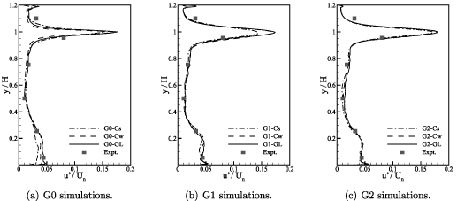
Figure 4. Normalised streamwise velocity fluctuation profiles, obtained at  0.5.
0.5.
Download figure:
Standard image High-resolution image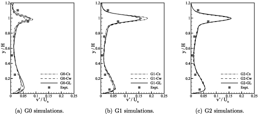
Figure 5. Normalised vertical velocity fluctuation profiles, obtained at  0.5.
0.5.
Download figure:
Standard image High-resolution imageThe mean concentration profiles, recorded at  0.05,
0.05,  0.5, and
  0.95, and the associated root mean squared (rms) concentration fluctuation profiles, are shown in figure 6, along with the experimental data. The prediction of the mean concentration at all three measurement locations is poor on G0, particularly for G0-Cs. For a constant emission rate of the tracer gas at the cavity base, the gross over-prediction of the mean tracer gas concentration in the G0 simulations implies that the tracer gas is not adequately removed from the cavity. The mean concentration predictions on G1 and G2 are in much better agreement with the experimental data, with the G2 cases offering some improvement over G1. The G0 simulations show reasonable prediction of the rms concentration fluctuation at
  0.05, with poor predictions elsewhere. The G1 and G2 simulations again show superior agreement with the experimental data.

Figure 6. Concentration statistics obtained at various streamwise locations within the cavity.
Download figure:
Standard image High-resolution imageA measure of the performance of the simulations in predicting flow quantities can be obtained by examining the correlation between an observed quantity, C0, and the predicted value,  . Figure 7 shows scatter plots of the predicted mean concentration against the observed mean concentration for each simulation. The simulations are grouped by subgrid-scale model type in each image to highlight the effect of the grid resolution on the simulation performance. For the Smagorinsky model, predictions greater than a factor of two of the observed values are present on G0, whereas all G1 and G2 data from the Smagorinsky cases reside within a factor of two of the experimental data. All cases show a bias towards over-prediction of the mean concentration, with the magnitude of the over-prediction decreasing with increasing grid resolution. For the WALE and G-L models, the G0 simulations again show a bias towards over prediction of the mean concentration, but the G2 cases provide excellent correlation with the reference data.
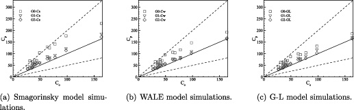
Figure 7. Scatter plot of predicted against observed mean concentration values at mid-span of the rig.
Download figure:
Standard image High-resolution imageA quantitative assessment of simulation accuracy can be obtained through analysis of several indicators (Chang and Hanna 2004, Hanna and Chang 2012). These indicators are as follows. The fraction of predictions within a factor of two of observation (FAC2) is given by

The fractional bias (FB) is defined as

where an overline denotes averaging over all considered values. The FB yields a measure of the mean relative bias in the data. The root normalised mean square error (RNMSE) is given by

which provides an indication of the relative scatter of the data. The geometric mean bias (MG) is defined as
which estimates the mean relative bias. The geometric variance (VG) is defined as
which estimates the relative scatter of the data.
Each indicator has a target value, and a range within which the simulation data can be considered acceptable. The values are computed over all 18 points where experimental data were recorded, the locations of which are shown in figure 1. Table 1 lists the values for these indicators for the mean concentration field. Underlined values indicate a violation of the acceptable range of the metric in question. Violations of FB and MG are reported for each of the G0 calculations, and no violation of any indicator is reported on G1 and G2. For each subgrid-scale model, the G2 simulations show marginal improvements in the indicators when compared to the counterpart G1 simulations.
Table 1. Performance metrics for mean concentration statistics in the simulations. Underlined values denote violation of the acceptable range for the metric.
| Metric | FAC2 | FB | RNMSE | MG | VG |
|---|---|---|---|---|---|
| Target | 1 | 0 | 0 | 1 | 1 |
| Range |
 0.5 0.5 | ] −0.3, 0.3 [ |
 1.2 1.2 | ] 0.7, 1.3 [ |
 4 4 |
| G0-Cs | 0.80 | −0.54 | 0.54 | 0.57 | 1.39 |
| G0-Cw | 0.93 | −0.49 | 0.42 | 0.61 | 1.30 |
| G0-GL | 0.93 | −0.43 | 0.35 | 0.64 | 1.23 |
| G1-Cs | 1.0 | −0.21 | 0.20 | 0.81 | 1.05 |
| G1-Cw | 1.0 | −0.15 | 0.12 | 0.86 | 1.03 |
| G1-GL | 1.0 | −0.17 | 0.15 | 0.84 | 1.03 |
| G2-Cs | 1.0 | −0.2 | 0.16 | 0.82 | 1.05 |
| G2-Cw | 1.0 | −0.15 | 0.11 | 0.86 | 1.03 |
| G2-GL | 1.0 | −0.14 | 0.10 | 0.87 | 1.02 |
The indicators are also computed for the rms concentration fluctuation, and are listed in table 2. Violations of FB are noted for G0-Cs, and G0-Cw, and a violation of MG is reported for G0-Cs.
Table 2. Performance metrics for rms concentration fluctuation statistics in the simulations. Underlined values denote violation of the acceptable range for the metric.
| Metric | FAC2 | FB | RNMSE | MG | VG |
|---|---|---|---|---|---|
| Target | 1 | 0 | 0 | 1 | 1 |
| Range |
 0.5 0.5 | ] -0.3, 0.3 [ |
 1.2 1.2 | ] 0.7, 1.3 [ |
 4 4 |
| G0-Cs | 0.73 | −0.46 | 0.29 | 0.62 | 1.37 |
| G0-Cw | 0.8 | −0.31 | 0.38 | 0.73 | 1.29 |
| G0-GL | 0.8 | −0.23 | 0.42 | 0.78 | 1.26 |
| G1-Cs | 1.0 | −0.17 | 0.18 | 0.84 | 1.08 |
| G1-Cw | 1.0 | −0.1 | 0.19 | 0.9 | 1.04 |
| G1-GL | 1.0 | −0.05 | 0.21 | 0.95 | 1.04 |
| G2-Cs | 1.0 | −0.14 | 0.14 | 0.87 | 1.05 |
| G2-Cw | 0.93 | −0.12 | 0.10 | 0.88 | 1.07 |
| G2-GL | 1.0 | −0.10 | 0.11 | 0.9 | 1.03 |
The analysis of the flow statistics shows that no simulation on G0 produces reliable flow statistics, and no further analyses of the G0 simulations will be presented here. In contrast, all G1 and G2 simulations produce data which, from a statistical performance perspective, are acceptable. The following section further analyses the fluid dynamics present in the G1 and G2 calculations.
5. Flow statistics
Streamlines of the mean velocity field within the cavity are shown in figure 8 for G1-GL and G2-GL. The mean velocity field of these simulations (and all others on G1 and G2) display common features; a large primary recirculation vortex can be seen in the centre of the cavity, along with smaller vortices located at the bottom of the leeward wall, at the bottom of the windward wall, and at the top of the leeward wall. The shear layer which develops over the top of the cavity can clearly be seen in both cases, with the shear layer thickness increasing with streamwise distance from the upstream cavity edge.
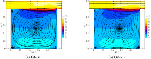
Figure 8. Streamlines of mean velocity in the cavity recorded at mid-span of the computational domain.
Download figure:
Standard image High-resolution imageA measure of the cavity shear layer thickness can be obtained from the vorticity thickness, defined as

where the velocity gradient is computed in the region encompassing the shear layer, 0.8  . Here the cavity shear layer is approximated as a single stream shear layer, such that
  in equation (13). The estimated vorticity thickness of the predicted shear layers are shown in table 3 for all simulations. On both G1 and G2, the Smagorinsky model simulation predicts the thinnest shear layer at
  0.5, whilst the WALE and G-L simulation produce data which is closely matched.
Table 3. Normalised vorticity thickness of the cavity shear layer at  .
.
| Model |

|
|---|---|
| G1-Cs | 0.084 |
| G1-Cw | 0.091 |
| G1-GL | 0.095 |
| G2-Cs | 0.081 |
| G2-Cw | 0.094 |
| G2-GL | 0.098 |
As shear layers are hypersensitive to the conditions from which they develop, it is important to quantify the flow conditions upstream of the cavity. Figure 9 shows the predicted mean streamwise velocity profiles of the boundary layer immediately upstream of the cavity edge ( ). On G1 (figure 9(a)), simulations G1-Cw and G1-GL produce identical laminar boundary layer velocity profiles at the upstream cavity edge, but case G1-Cs produces a boundary layer which is considerably thicker than the other two simulations. On G2 (figure 9(b)) the same trends are observed, but the predicted boundary layers are much thinner than those obtained on G1. The boundary layer thickness, δ, is defined as the vertical location where the local mean streamwise velocity attains a value of 99% of the freestream value. The computed boundary layer thickness from all simulations are outlined in table 4. For a given calculation on G2, the predicted boundary layer thickness is approximately 20% smaller than for its G1 counterpart calculation. The momentum thickness of the boundary layer is computed from,
  , and is shown in table 4 for each case. The predicted momentum thickness of the boundary layer increases when the Smagorinsky model is employed, on both grids. For a particular grid resolution all of the WALE model cases, and the Germano-Lilly model calculation, predict matching values of boundary layer momentum thickness. In all simulations the shape factor of the boundary layer has a value of approximately 2, indicating that the boundary layer at the upstream cavity edge is laminar in nature.
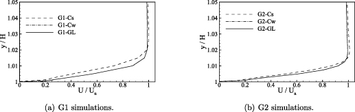
Figure 9. Normalised mean streamwise velocity profiles obtained at  −0.02, upstream of the cavity edge.
Download figure:
Standard image High-resolution imageTable 4. Properties of the boundary layers at the edge of the leeward channel  . The frequency f is that of the most amplified disturbance in the cavity shear layer, obtained from St
 (Michalke 1964).
| Simulation |

|

| f (Hz) |
|---|---|---|---|
| G1-Cs | 2.11 | 3.05 | 6.1 |
| G1-Cw | 1.82 | 2.4 | 7.44 |
| G1-GL | 1.82 | 2.4 | 7.44 |
| G2-Cs | 1.56 | 2.09 | 8.6 |
| G2-Cw | 1.44 | 1.86 | 9.61 |
| G2-GL | 1.44 | 1.86 | 9.61 |
Given that the cavity shear layer develops from laminar conditions the frequency, f, of the most amplified disturbance in the shear layer can be obtained from the Strouhal number of the flow, St  , if the cavity shear layer is approximated as a single stream shear layer (Michalke 1964). The most amplified disturbance frequency is given in table 4 for all cases. This frequency corresponds to the frequency of the Kelvin–Helmholtz (K-H) instability in the shear flow (Michalke 1964). As the shear layer evolves over the cavity, the growth of the layer is dictated by interactions between K-H vortices. This process is driven by the saturation of subharmonics of the primary instability (Ho and Huang 1982). Evidence for the presence of large-scale K-H type structures in the cavity shear layer can be obtained from instantaneous plots of spanwise vorticity,
  , shown in figure 10. The spanwise vorticity maps presented here are normalised by the cavity height, and the reference velocity, Un
. In the map obtained from G1-GL, large, K-H vortices are present in the cavity shear layer at
, shown in figure 10. The spanwise vorticity maps presented here are normalised by the cavity height, and the reference velocity, Un
. In the map obtained from G1-GL, large, K-H vortices are present in the cavity shear layer at  0.25, 0.35. Downstream of
  0.55 small scales of spanwise vorticity are present in the shear layer, indicating that the flow has become turbulent. The transition to turbulence in the shear layer is precipitated by pairing interactions between the K-H vortices (Huang and Ho 1990). The contour map obtained from G2-GL also shows laminar vortices present in the shear layer, upstream of
  . Downstream of this location the shear layer has undergone the transition to turbulence, and large-scale coherent turbulent structures are present in the layer (Brown and Roshko 1974). In these images it can be seen that the shear layer in G2-GL undergoes a more rapid evolution than its G1-GL counterpart, because the momentum thickness of the boundary layer at the upstream edge of the cavity is smaller in G2-GL than in G1-GL. The more rapid evolution of the G2 simulations can be quantified through interrogation of the average streamwise location at which vortex interaction events occur. The pairing parameter,
  , where
  is the velocity ratio parameter (Huang and Ho 1990), is commonly used to ascertain the evolution of the vortex structure in a shear layer which originates from laminar upstream conditions. Approximating the cavity shear layer as a single-stream shear layer yields
  1. The roll-up of the shear layer into K-H vortices will occur at
  , the first generation of vortex interactions will occur at
  , the second generation will occur at
  and so on. Experimental and numerical investigations have shown that the transition to turbulence in the shear layer typically occurs with the second generation of vortex interactions. Profiles of the streamwise distribution of the rms streamwise velocity fluctuation along the horizontal plane at the top of the USC (
 1) can be used to deduce the occurrence of vortex interactions in the shear layer (Browand and Latigo 1979, McMullan et al
2015). These profiles are shown in figure 11(a) for the G1 cases, and figure 11(b) for the G2 cases. The profiles for all simulations show similar features; the quantity increases to a shoulder in the profile, followed by a second local maximum. Towards
1) can be used to deduce the occurrence of vortex interactions in the shear layer (Browand and Latigo 1979, McMullan et al
2015). These profiles are shown in figure 11(a) for the G1 cases, and figure 11(b) for the G2 cases. The profiles for all simulations show similar features; the quantity increases to a shoulder in the profile, followed by a second local maximum. Towards  the quantity increases as the shear layer interacts with the windward wall. For all cases the shoulder in the profile corresponds well to a pairing parameter value of
  4, showing that this feature is caused by the first generation of pairing between vortices. The second maximum in the profiles occurs at
  8; this is the second generation of pairings that precipitates the transition to turbulence in the shear layer. For a given grid, the profiles extracted from the WALE and G-L simulations are closely matched, whilst the peaks in the profiles extracted from the Smagorinsky model simulations are shifted downstream. The profiles from the G2 simulations show that the shear layers evolve more rapidly on this grid, when compared to the G1 cases. The delay in the evolution of the shear layer in the G1 cases is caused by the larger momentum thickness of the boundary layer departing the upstream cavity edge. Similarly, the Smagorinsky model predictions are delayed when compared to the WALE and G-L cases for a given grid, because the momentum thickness of the upstream boundary layer is 15% higher on G1, and 8.3% higher on G2, as noted in table 4.
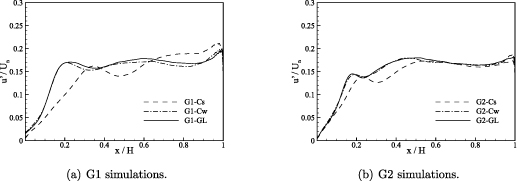
Figure 10. Contour map of normalised instantaneous spanwise vorticity within the cavity. Visualisations captured at an arbitrary time instant.
Download figure:
Standard image High-resolution image
Figure 11. Normalised streamwise velocity fluctuation profiles along the upper edge of the cavity,  1.
1.
Download figure:
Standard image High-resolution imageFigure 12 shows PSD plots of the streamwise velocity fluctuation at  = (0.05, 0.95) - a location which resides at the lower edge of the cavity shear layer. In these plots, the curves are shifted on the vertical axis for clarity. Case G1-Cs shows a well-defined peak in the spectrum at a frequency of 3.4 Hz. The peak frequency is approximately a factor of two smaller than the most amplified disturbance frequency outlined in table 4, hence the peak is associated with the passage of vortical structures which are the first subharmonic of the cavity shear layer primary instability. The spectra from G1-Cw and G1-GL show no evidence of this peak; instead the slope of the spectra approach a -5/3 roll-off, which indicates the presence of a fully turbulent shear layer. The spanwise vorticity map of G1-GL in figure 10(b) shows that small-scale vorticity is present in the shear layer at
  , confirming that the flow has become turbulent at this streamwise location. For the G2 simulations there are no peaks observed in any of the spectra—the curves approach a
  roll-off which demonstrates that each simulation has become turbulent at the probe location.
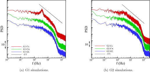
Figure 12. PSD curves of the streamwise velocity fluctuation, recorded at  . Spectra are shifted vertically on the image for clarity.
Download figure:
Standard image High-resolution imageJoint probability density functions (JPDFs) of the streamwise and vertical velocity fluctuations  recorded at
  are shown in figure 13. The axes divide the
  plane into four quadrants, which denote the following contributions to the momentum flux (Willmarth and Lu 1975, Shaw et al
1983):
plane into four quadrants, which denote the following contributions to the momentum flux (Willmarth and Lu 1975, Shaw et al
1983):
-
 : outward interaction
 -
: ejection or burst
-
: inward interaction
-
: sweep or gust


Figure 13. Joint probability density functions of streamwise and vertical velocity fluctuations, recorded at  .
.
Download figure:
Standard image High-resolution imageFor G1-Cs, sweep events are the most probable, and the magnitude of the fluctuations is not far beyond zero. Both outward interaction, and ejection events, also provide significant contributions to the momentum flux. As noted above, the cavity shear layer is laminar at this location in G1-Cs, hence the fluctuations present in the layer will be the result of large scale motions caused by the K-H vortices. The JPDFs of G1-Cw, G2-Cs, and G2-Cw, are markedly similar (as are those of G1-GL and G2-GL, not shown here); sweep events transport high-momentum fluid downwards, and ejections transport low-momentum fluid upwards. These JPDFs arise as a result of the dynamics of the turbulent vortex structures in the cavity shear layer, where pairing interactions between the structures entrains high-momentum fluid towards the low-speed side of the layer, and vice versa (Dimotakis 1986, Huang and McMullan. 2021). The JPDFs of velocity fluctuations are analysed at intervals of 0.1 H along the upper edge of the cavity—it is found that G1-Cs attains the same distribution as the other simulations downstream of  0.6, coinciding with the establishment of a fully turbulent shear layer. It is important to note that the current simulations originate from laminar upstream conditions, and as such the evolution of the cavity shear layer is markedly different to configurations where the upstream conditions are based on atmospheric boundary layers (Cui et al
2004, Cheng and Liu 2011, Kikumoto and Ooka 2012), where large turbulent structures present in the upstream flow gives rise to a cavity shear layer quadrant analysis that shows ejections are more common than sweep events.
0.6, coinciding with the establishment of a fully turbulent shear layer. It is important to note that the current simulations originate from laminar upstream conditions, and as such the evolution of the cavity shear layer is markedly different to configurations where the upstream conditions are based on atmospheric boundary layers (Cui et al
2004, Cheng and Liu 2011, Kikumoto and Ooka 2012), where large turbulent structures present in the upstream flow gives rise to a cavity shear layer quadrant analysis that shows ejections are more common than sweep events.
The results presented here show that the simulated fluid dynamics are markedly different between G1 and G2. For the intermediate grid, the Smagorinsky model has a deleterious influence of the predicted flow, whilst the WALE and Germano-Lilly models produce reasonable predictions. Increasing the grid resolution for the fine grid results in a diminished influence of the subgrid-scale model, and an improvement in the predicted fluid dynamics. The results here indicate that an improved grid resolution has a more substantial effect on the overall accuracy of the simulation, than in improvement in subgrid-scale modelling methodology on a less well-refined grid.
6. Tracer gas dispersion
Instantaneous maps of the concentration field in G1-GL and G2-GL are shown in figure 14, with the images captured at the same time instant as the respective spanwise vorticity plots of figure 10. The tracer gas is transported towards the leeward wall by the cavity vortex, where it subsequently moves upwards towards the top of the cavity. The tracer gas then interacts with the cavity shear layer, and it is mixed with freestream air. Not all of the tracer gas is entrained into the shear layer and removed from the cavity; instead some of the tracer gas is recirculated into the cavity at the windward wall. The map of G1-GL, shows high levels of tracer gas concentration extending up the leeward wall, and into the cavity shear layer. The tracer gas is entrained into the shear layer by the K-H vortex structures visible in figure 10(a). This entrainment occurs in the interconnecting braid regions between the laminar vortices, with little mixing occurring in the laminar vortex cores. Once the cavity shear layer undergoes the transition to turbulence (downstream of  0.55 in this particular instant in time), the tracer gas is mixed with freestream air in the shear layer. The delayed roll-up of the shear layer in G1-GL described above reduces the overall entrainment appetite of the cavity shear layer, as fewer vortical structures are present in the shear layer. This results in a reduction in the the amount of tracer gas removed from the USC, and consequently an over-prediction of the mean tracer gas concentration within the cavity on G1, as observed in figure 6. For case G2-GL, the tracer gas jet breaks down rapidly towards the leeward wall, and the earlier roll-up of the G2 shear layer into discrete vortices enhances the entrainment of tracer gas into the shear layer. In addition, the more rapid transition to turbulence in the G2 cavity shear layer promotes the efficient mixing and removal of the tracer gas from the cavity. The improved prediction of the cavity shear layer dynamics on G2 leads to an accurate prediction of the mean concentration statistics shown in figure 6.

Figure 14. Contour map of normalised instantaneous tracer gas concentration within the cavity. Visualisations captured at the same time instant as the respective spanwise vorticity plot in figure 10.
Download figure:
Standard image High-resolution imageContour maps of the vertical concentration flux,  , are shown in figure 15 for G1-Cs, G1-Cw, G2-Cs, and G2-Cw. The maps obtained from G1-GL and G2-GL are very similar to G1-Cw, and G2-Cw respectively, and are not shown here. All four simulations show a strong vertical flux near to the line source at the base of the cavity, which is angled towards the leeward wall due to the circulation of the primary cavity vortex. Each simulation also shows a region of vertical flux near the windward wall, caused by the mixing of the recirculated tracer gas with ambient air entrained from the freestream. Each simulation also shows a strong vertical concentration flux in the cavity shear layer. The distribution of
  is broadly similar to other studies of pollutant dispersion in a cavity (Li et al
2010). The behaviour of the vertical concentration flux along the streamwise extent of the cavity shear layer is closely linked to the evolution of the shear layer described above. From zero concentration flux at the upstream edge of the cavity, the quantity increases to maximum at approximately the location where the first pairing interaction between K-H vortices. The vertical concentration flux remains elevated along the remainder of the shear layer. For G1-Cs, the streamwise location of the maximum in
is broadly similar to other studies of pollutant dispersion in a cavity (Li et al
2010). The behaviour of the vertical concentration flux along the streamwise extent of the cavity shear layer is closely linked to the evolution of the shear layer described above. From zero concentration flux at the upstream edge of the cavity, the quantity increases to maximum at approximately the location where the first pairing interaction between K-H vortices. The vertical concentration flux remains elevated along the remainder of the shear layer. For G1-Cs, the streamwise location of the maximum in  is shifted downstream when compared to G1-Cw. Similarly, the evolution of
  is delayed on G1 when compared to G2, owing to the larger momentum thickness of the upstream boundary layer as outlined in table 4. The delay in the evolution of the shear layer in G1 produces a reduction in the vertical concentration flux within the shear layer, reducing the removal of the tracer gas from the cavity.

Figure 15. Contour maps of turbulent vertical concentration flux,  , recorded at mid-span of the domain,
  .
.
Download figure:
Standard image High-resolution imageConcentration probability density functions (PDFs) are presented from three regions of interest in the cavity; mid-height of the leeward wall,  (0.05, 0.5), the centre of the cavity in the vicinity of the shear layer, (
 (0.5, 0.95), and mid-height of the windward wall, (
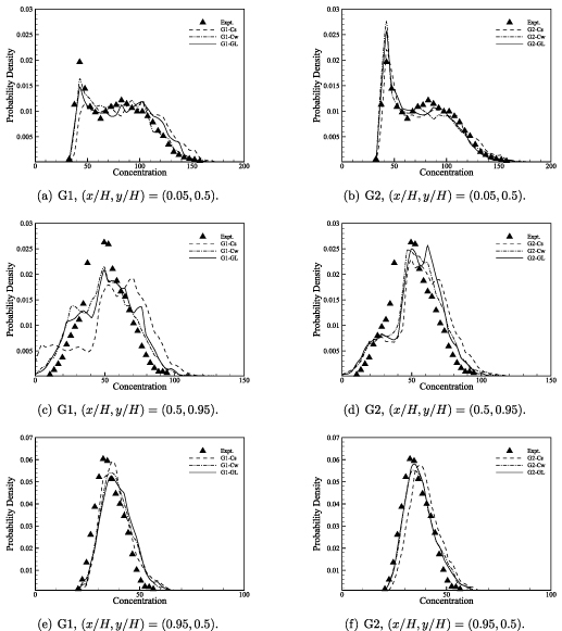
 (0.95, 0.5). The PDFs obtained from the G1 and G2 simulations are shown in figure 16. The experimental data are shown as symbols, and the simulation data are presented as line plots. Figure 16(a) shows the concentration PDF at
  (0.05, 0.5) from the G1 calculations. The peak in the experimental data at
  is not present in G1-Cs, although the range of concentrations observed at this measurement location is in good agreement with the experimental data. Cases G1-Cw and G1-GL capture the peak at
  , although the magnitude of the probability density in lower than the experimental data. The range of concentrations observed, and the general distribution of the PDF in G1-Cw and G1-GL are in extremely good agreement with the experiment.
Figure 16. Concentration probability density function distributions at selected measurement stations. All measurements obtained at mid-span of the domain.
Download figure:
Standard image High-resolution image
The concentration PDFs at  (0.05, 0.5) on G2 are shown in figure 16(b). The Smagorinsky model prediction has improved substantially on this grid, with the most probable concentration now correctly captured. All three simulations on G2 produce data which agree exceptionally well with the experimental data, and the over-prediction of the probability density of the most probable concentration is consistent with previous LES studies (Kikumoto and Ooka 2018). The concentration PDFs at the top of the cavity, (
 (0.5, 0.95), in G1 are shown in figure 16(c). Case G1-Cs predicts a bi-modal distribution, with a broad peak at low concentration values. Similar distributions are present in G1-Cw and G1-GL, with a narrow separation between the peaks. No simulation on G1 produces good agreement with the experimental data, due to the delayed evolution of the cavity shear layer described above. The PDFs obtained at (
 (0.5, 0.95) on G2 are shown in figure 16(d). All simulations now offer improved predictions when compared to G1, but the predicted distributions also show evidence for a bi-modal type distribution that was not observed in the experiment. The most probable concentration is, however, well-predicted in all three G2 calculations.
At ( (0.95, 0.5). the concentration PDFs from G1 (figure 16(e)) yield good predictions from all three simulations, but the distributions are shifted to higher values of the normalised concentration compared to the experiment. This discrepancy arises from the fact that insufficient quantities of tracer gas are removed from the cavity by the shear layer, owing to the poor prediction of the shear layer evolution on the intermediate grid. The PDFs from the G2 cases, shown in figure 16(f), show substantially improved agreement with the experiment—the most probable concentration, and the range of observed concentrations, are accurately captured in G2-Cw and G2-GL. The improvement in the PDF distribution arises from the improved entrainment and mixing of the tracer gas in the cavity shear layer, which therefore results in adequate removal of the tracer gas from the cavity.
Given that all G1 and G2 simulations satisfied the performance metrics in tables 1 and 2, the marked differences in the concentration probability density functions indicate that caution must be exercised when relying upon metric indicators to assess the quality of a simulation.
7. Conclusions
LES of tracer gas dispersion within a cavity has been performed. The flow originated from laminar upstream conditions, resulting in a shear layer which undergoes a transition to turbulence as it develops over the cavity. A systematic study of the effects of grid resolution, and subgrid scale model, on the tracer gas dispersion has shown that the intermediate and fine grids satisfy quantitative metrics for acceptable simulation of the mean, and rms concentration fields. Analysis of the fluid mechanical processes present in the simulation reveals that the prediction of the tracer gas dispersion is heavily influenced by the evolution of the simulated cavity shear layer. On an intermediate resolution grid the standard Smagorinsky model over-predicts the upstream boundary layer thickness, which results in a delayed development and evolution of the shear layer. The transition to turbulence in the shear layer occurs too far downstream, inhibiting the mixing and subsequent removal of the tracer gas from the cavity. WALE model, and Germano-Lilly model simulations on the intermediate grid are improved when compared to the standard Smagorinsky model, but remain deficient when compared to fine grid simulations. The concentration probability density functions produced on the intermediate grid show reasonable agreement with the experimental data, but the fine grid simulations offer extremely good agreement with the reference data.
The results presented in this paper clearly demonstrate that, despite satisfying the performance metrics, the intermediate grid calculations suffer from deficiencies which limit their ability to accurately predict tracer gas dispersion in a cavity. The standard Smagorinsky model, commonly used in urban environment studies, offers poor predictions of the mixing processes on an intermediate grid. Utilising enhanced subgrid-scale modelling methodologies can offset some of these deficiencies, but cannot surmount the fundamental constraints imposed by the grid resolution. In order to produce good predictions of the fluid mechanical processes governing tracer gas dispersion in a cavity, It is shown that performing simulations on a fine grid with the Smagorinsky model is preferable to using a more complex subgrid-scale model on a less well-refined grid. Future articles will expand this work for stratified flows in the cavity, and study the effects of an upstream turbulent flow on the dispersion of the tracer gas.
Acknowledgments
This research was performed on ALICE2, the University of Leicester High Performance Computing Service. The research was supported through a Royal Academy of Engineering / Leverhulme Trust Research Fellowship, Grant No. LTRF1920\16\38.