

Abstract
For both real fish and bionic fish, a rigid anterior portion is necessary for certain functions. How does the rigid anterior portion affect the locomotion of the flexible plate? Is it true that the rigid portion is redundant? It is lack of clear cognition on these questions. In this paper, the self-propulsion of the rigid-flexible composite plate is studied numerically. We suppose that the forces are exerted on the junction point to maintain a given pitch motion of the rigid portion, the deformation of the flexible portion is consequent. The ratio between the lengths of the flexible portion and the rigid portion is changed to model the composite plate, and the effect of the stiffness of the flexible plate is investigated. It is found that the propulsive velocity and the Froude efficiency actually decrease following the increasing proportion of the rigid plate. However, the conclusion is different as the elastic energy stored in the flexible plate is considered. We find that the case with larger flexible portion is efficient for the ultra-soft posterior plate, while the case with smaller flexible portion is efficient for the stiff posterior plate. It happens to coincide with the swimming behavior of live fish. The hydrodynamic force at the tail is hindering the propulsion of the plate, which means that the motion of the tail plays a decisive role on the force distribution on the plate, rather than the thrust only produced at the tail. We think that the short ultra-soft membrane at the tail of the real fish is an important feature to improve its swimming behavior. It is expected that the study in this paper will give a further insight into the mechanism of the locomotion of fish and give some implications for the design of the soft bionic fish.
Export citation and abstract BibTeX RIS

Original content from this work may be used under the terms of the Creative Commons Attribution 4.0 license. Any further distribution of this work must maintain attribution to the author(s) and the title of the work, journal citation and DOI.
Recommended by Professor Hyung Jin Sung
1. Introduction
After evolution of thousands of years, fish can swim effectively, powerfully and agilely. The design of autonomous underwater vehicles (AUVs) could greatly benefit from learning the swimming behavior of fish, which bend in similar ways within a highly predictable range of characteristic motions (Lucas et al 2014) visually. To facilitate the updating of the underwater biomimetic pusher from appearance to spirit, the research on the physical mechanism of the swimming behavior of fish is of great concern. Although a lot of works have been done to study the swimming behavior of fish, but it is still not completely clear (Gemmell et al 2015, 2016). The BCF (body and/or caudal fin) mode is the most common swimming mode of fish, which is efficient and has huge application potential in underwater biomimetic pusher.
In BCF mode, fish propels itself by wiggling the posterior part, while the anterior part acts as a rigid structure (Lindsey 1978, Sfakiotakis et al 1999). In the traditional sense, the undulation of the posterior part of the fish is the power source to propel itself, while the anterior part maybe hindering propulsion. So, the previous researches had focused on the flexible structure, which only model the fish in anguilliform mode (Borazjani and Sotiropoulos 2008) or the posterior part of the fish (Borazjani and Sotiropoulos 2010, Abbaspour and Najafi 2018). However, Lucas et al (2020) found that the motion of the rigid anterior part could generate suction to increase propulsive force, which accounted for about quarter of the total thrust. The hydrodynamics of the onefold flapping rigid or flexible plate have been studied extensively, which will be introduced in next context. However, the research on the hydrodynamics of the rigid-flexible composite structure is still in vacuum at present, which maybe give a further understanding to the locomotion in BCF mode.
The locomotion of the fish is a typical fluid-solid coupling problem, which involves a complex balance of different force: muscles produce force to move the body; the body has inertial, elastic, and damping properties that may aid or oppose the muscle force; and the environment produces reaction forces back on the body (Tytell et al 2010). Compared with live fish, the flexible structure is a better choice to study the complete fluid-solid coupling process in the locomotion of fish, whose kinematic and dynamic parameters can be controlled. In view of the simple geometry of the waving plate or bar, it has been widely used to model the undulation of fish, and some important progresses have been published. Lighthill (1960) and Wu (1961) indicated that the backward propagating undulation on the plate could product propulsive force and the kinematics of the tail was the key factor.
Alben et al (2012) found that, the length and rigidity affected the propulsion of the plate dramatically. The resonant-like peaks in the swimming speed were the functions of the foil length and rigidity. Olivier and Dumas (2016a, 2016b) had studied the propulsion of flapping flexible wing, the inertia-driven and the pressure-driven deformations were identified. And an additional feathering effect, the rigid feathering effect, was presented as the pressure-to-inertia ratio was high. Yin and Luo (2010) and Hua et al (2013) had studied the locomotion of the flexible plate driven by the heaving motion of the leading edge, and it was found that the resonance was beneficial to elevate the thrust and propulsive efficiency. Zhang et al (2017) found that, the resonance could significantly improve the thrust force and efficiency at low and intermediate mass ratio, while the effect of the resonance was unconspicuous at high mass ratio. Ramananarivo et al (2011) pointed out that, rather than the resonance, the phase dynamics in the oscillator model was the key factor to improve the self-propulsion of the plate. Wu (2020) indicated that whether the resonance or the phase dynamics was the key factor to improve the self-propulsion was related to the driving mode of the plate.
In the nature, fish in BCF mode is usually not fully flexible, still has a rigid head at least. In engineering, the anterior of the bionic fish should be rigid to install some equipment. In a word, neither the live fish nor the bionic fish is driven at nose. So, the self-propulsion of the flexible plate driven by the motion of the leading edge cannot express the hydrodynamics of a whole fish. In this paper, the self-propulsion of the rigid-flexible composite plate was investigated, which modeled the fish in BCF swimming mode. The rigid plate was corresponding to the anterior part, while the flexible plate was corresponding to the posterior part.
Irrespective of the complex muscle model in McMillen et al (2008), we only gave the pitching motion of the rigid plate, which could capture the main features of the locomotion of the fish (Shelton et al 2014, Lim and Lauder 2016, Tytell et al 2016). To study the effect of the muscle force at different location of fish on its locomotion, we supposed that the external forces only exerted on the rigid-flexible junction point, which was also truthfulness for flexible pusher of the underwater vehicles. The propulsive speed and efficiency, the thrust and the flow structure were investigated here. It was expected that the study on the self-propulsion of the composite plate would give a further insight into the mechanism of the locomotion of fish. It also has implications for the design of the soft bionic fish, which is usually consist of the rigid forepart contain motor and the flexible posterior made from new material.
2. Physical problem and mathematical formulation
A two-dimensional model of the rigid-flexible composite plate is considered. As shown in figure 1, XOY is the inertial coordinate system. The length of the flexible part is lf
, and the length of the rigid part is lr
. The rigid plate swings around the head point o, and  is the swinging angle. c is the connect point of the rigid plate and the flexible plate, and b is the tail point of the plate. The composite plate is propelling itself in the quiescent flow, while Up
is the cruise speed.
is the swinging angle. c is the connect point of the rigid plate and the flexible plate, and b is the tail point of the plate. The composite plate is propelling itself in the quiescent flow, while Up
is the cruise speed.
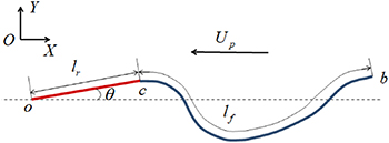
Figure 1. The sketch of the model for the locomotion of the rigid-flexible composite plate.
Download figure:
Standard image High-resolution imageThe motion of the flexible plate is governed by the nonlinear partial differential equation

where s is the Lagrangian coordinate along the flexible plate, and the junction c is its origin.
r
is the position vector in the inertial coordinate system,  is mass per unit length of the plate.
  is the tension with Eh being the stretching rigidity, h is the thickness of the plate, and EI is the bending rigidity.
F
f
is the force vector exerted on the plate, which is calculated with the relative velocity vector between the predicted flow velocity and the velocity of the plate Pinlli et al (2010), as shown in equation (17). The boundary conditions at the tail point b are
is the tension with Eh being the stretching rigidity, h is the thickness of the plate, and EI is the bending rigidity.
F
f
is the force vector exerted on the plate, which is calculated with the relative velocity vector between the predicted flow velocity and the velocity of the plate Pinlli et al (2010), as shown in equation (17). The boundary conditions at the tail point b are

While the boundary conditions at the junction c are related to the motion of the rigid plate.
To imitate the motion of the anterior of the fish, we suppose the head point o can only move in the X direction. The swing of the rigid plate is given as  , where
  and f are the amplitude and frequency of the swing respectively. The first derivative of the displacement respect to s at point c can be calculated


Suppose the displacement of the head point c is (xc, yc ), we can express the displacement of the point on the rigid plate as


where sr is the Lagrangian coordinate along the rigid plate, whose origin is point o. The kinetic energy of the rigid plate can be deduced as

The forces exerted by the flexible plate on the rigid plate are denoted as Fcx, Fcy, Mcx and Mcy , which are corresponding to freedoms of the point c. No external force is acting on the head point, which is consistent with the truth that the fish cannot generate force at the nose. The pressure exerted by the fluid on the plate is p, which is a function of sr . The work done by the external forces can be expressed as
The swing of the rigid plate and the lateral motion of the point o is given, namely yc
,  and
and  is specified. So the dynamic governing equation of the rigid plate can be deduced using Lagrange equation

The boundary conditions of the flexible plate at the junction point c are

The incompressible Navier–Stokes equations are used to describe the flow dynamics


where U is the velocity vector, p is the pressure, ρ is the density of the fluid and v is the kinematic viscosity coefficient. The flow is initially quiescent. The velocity boundary condition for the fluid is imposed on the plate

The total length of the composite plate l = lr + lf
is fixed. The ratio between the length of the flexible plate to the total length l*
= lf
/l varies from 0.3 to 1. The frequency Reynolds number is defined as Ref
= fl2/ν and is fixed as 1 × 10⁴ here, which is applicable to simulate the fish swimming in the nature. The densities per unit length of the rigid plate and the flexible plate are the same, namely ρr
= ρl
. The mass ratio of the plate to the fluid is defined as  , which is fixed as 2 following previous research (Yin and Luo 2010, Hua et al
2013). w is the width of the plate, which is 1 by default here because the dynamics of the system have nothing to do with the width. To unify the dynamic characteristics of the flexible plate, the bending stiffness is expressed in the form
, which is fixed as 2 following previous research (Yin and Luo 2010, Hua et al
2013). w is the width of the plate, which is 1 by default here because the dynamics of the system have nothing to do with the width. To unify the dynamic characteristics of the flexible plate, the bending stiffness is expressed in the form  . The stretching stiffness
  , which is so large that the elongation of the plate can be ignored (Zhu 2002). The swing amplitude of the rigid plate is fixed as 0.2 rad, which is small enough to express the tiny wobble of the anterior part of the fish.
3. Numerical method and validation
3.1. Numerical method
The governing equations of the fluid-plate problem are solved numerically by the immersed boundary method (IBM) for the fluid flow and the finite element method for the motion of the flexible plate. When the IBM is used to treat flow-structure interaction, a reactive force is used to represent the effect of the structure on the fluid dynamics (Peskin 2002), namely a body force fb is added into the right hand of equation (11). The grids around the plate are uniform to use IBM, while the other grids are nonuniform to save the computing resources, as shown in figure 5(b). Equation (11) can be rewritten as

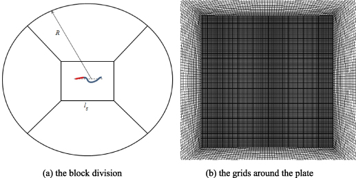
Figure 5. The grids around the plate and the computational domain. (a) The block division. (b) The grids around the plate.
Download figure:
Standard image High-resolution imagewhere  is the velocity vector of the grid, which is calculated using scaling method. A center point and two radii R1 and R2 are defined to implement the dynamic mesh computation. The design formulas are


The displacement of the grids is denoted as d g , and d o is the displacement of the head point of the plate. P is the initial position of the grid, and P 0 is the position of the center point of the circular computational domain.
The IBM is embedded into OpenFOAM (Jasak 2009) following the procedure proposed by Pinlli et al (2010) and Constant et al (2017). In Pinlli et al (2010), the hydrodynamic force in the right hand side of equation (1) is calculated as

where  is the velocity of the plate.
  is the velocity interpolated from the predicted flow velocity, namely Lagrangian–Euler interpolation

ϕ is the interpolation function, U * is the predicted velocity of the flow without the disturbance form the plate

The superscript n denote the value in previous time step.
After the Lagrangian force F f has been achieved, it can be transformed by a spreading operator C into the body force f b

Here, we just give a brief explanation of implementation process of the immersed boundary method. The detailed description can be consulted from the literature of Pinlli et al (2010). A second-order Gauss integration scheme with a linear interpolation for the face-centered value of the unknown is used for the divergence, gradient, and Laplacian terms in the governing equations. The second-order backward Euler method is adopted for time integration. Thus, the numerical discretization scheme gives second order accuracy in space and time.
The beam element is used to simulate the dynamics of the plate, and the element is uniformly distributed along the axis of the plate. After the dissociation of the finite element method, equation (1) can be expressed as a set of algebraic equations


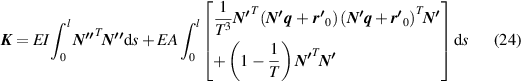

where M is the mass matrix, K is the stiffness matrix, F is the generalized force of the hydrodynamic force. r 0 is the original position of the point, which is added to the deformation of the plate to get the absolute position of the point. N is the shape function. q is the generalized displacement.
The Newmark-β method and the Newton–Raphson method are used to solve equation (23). The acceleration  and velocity
  at time t +Δt can be expressed as


The subscript t denotes the values at time t. Δt is the time step. The expressions of a0, a1, a2, a3, a4 and a5 are

where δ = 0.505 and β = 0.2525 are the Newmark coefficients. Equation (23) can be expressed as the non-linearity system of equations

According to Newton–Raphson method, equation (29) is solved iteratively
 is the first derivative of
  respect to
  . The initial value of the iteration is
  . As
. As  has been achieved,
  and
and  are calculated using equations (26) and (27).
4. Validation
To validate the numerical models and methods meticulously, the structure solver and the full FSI are validated separately.
4.1. Validation of the structural solver
As shown in figure 2, the structure solver is validated by calculating the large deflection of a cantilever beam with the length l and the bending stiffness of EI under a point force load F transversally at the free end. The results of the axial displacement u of the cantilever beam, the lateral displacement w and the deflection angle θ in three dimensionless form  ,
,  and θ are compared with the results of Mattiasson (2010) at different dimensionless force
  are shown in figure 3. The excellent agreement can be found.

Figure 2. The schematic diagram of the cantilever beam with a concentrated force at the free end.
Download figure:
Standard image High-resolution image
Figure 3. The axial displacement, transversal displacement and deflection angle at the free end of the cantilever beam. (a) Axial displacement. (b) Transversal displacement. (c) Deflection angle.
Download figure:
Standard image High-resolution image4.2. Validation of the FSI solver
The locomotion of the flexible plate has been simulated in Hua et al (2013). The leading-edge is forced to heave sinusoidally with amplitude A0 and frequency f in the vertical direction, which can be described as  . The frequency Reynolds number is 100, the heave amplitude of the leading edge
  . The propulsive velocity and efficiency of the flexible plate are used to compare with those in Hua et al (2013). The dimensionless propulsive velocity is defined as
  , where Up
is the propulsive velocity of the plate. The propulsive efficiency for the locomotion of flexible plate is expressed as (Kern and Koumoutsakos 2006)
, where Up
is the propulsive velocity of the plate. The propulsive efficiency for the locomotion of flexible plate is expressed as (Kern and Koumoutsakos 2006)

As shown in figure 4, the propulsive velocity and efficiency achieved in this paper match well with the results of Hua et al (2013). It is expected that the model and method in this paper can accurately simulate the locomotion of the flexible plate.
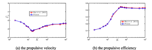
Figure 4. Comparison of the present result and those in Hua et al (2013). (a) The propulsive velocity. (b) The propulsive efficiency.
Download figure:
Standard image High-resolution image4.3. Grid testing
A circular computational domain has been used here, whose radius is R= 250 l. The division of the computational domain is shown in figure 5(a). The length of the sides of the rectangle is lg = 3 l, and the grids inside the rectangle domain is uniform, as shown in figure 5(b). The outer domain is divided using an O-type mesh. The size of the grids in the rectangle domain is dg , while the sizes of the other grids adjust following these sizes smoothly. To employ the IBM proposed in Pinlli et al (2010), the size of the grid on the plate used to solve the structure dynamics is as the same as that of the gird in the rectangle domain. Five different grids are used for the grid testing. The parameters of the case are l* = 0.5 and k= 30. The results are shown in table 1. It can be found that, the propulsive velocity and the propulsive efficiency at grid3 are accurate enough, namely, the effect of the grid refinement can be ignored. In this paper, the parameters for grid3 are used for all cases.
Table 1. The result for different grids.
| Grid1 | Grid2 | Grid3 | Grid4 | Grid5 | |
|---|---|---|---|---|---|
| dg | 0.005 | 0.0067 | 0.01 | 0.0133 | 0.02 |

| −1.204 | −1.211 | −1.214 | −1.214 | −1.223 |
| η | 40.27% | 40.74% | 41.35% | 41.33% | 42.61% |
5. Results and discussions
In this section, we present some typical results on the dynamics of the composite flexible plate. The stiffness of the flexible plate is in the range of 10 < K < 500, where the flexible plate moves forward in Hua et al's research (2013).
5.1. The propulsive velocity and efficiency
Figure 6 shows the propulsive velocity of the composite plate. For l*= 0.3 ∼ 0.6, the propulsive velocity increases following the stiffness and tends to be stable finally. For l*= 0.7 ∼ 1, the propulsive velocity increases following stiffness in the range of K< 60, then slightly decreases in the range of K> 60 and finally tends to be stable. For arbitrary K, the propulsive velocity increases following increasing l*, which means that the anterior rigid part of the composite plate actually produces smaller thrust than the flexible plate. It is worth mentioning that the resonance effect is not observed in the locomotion of the composite plate driving by pitch motion, which has been mentioned in Hua et al (2013) for a flexible plate driving by heave motion of the leading edge. It may be due to the pitching motion make the plate have an attack angle, which induce a large enough gradient at the tip (Lighthill 1960). Figure 7 shows the Froude efficiency of the composite plate. For arbitrary l*, the Froude efficiency increases following the increasing stiffness and finally tends to be stable. For arbitrary stiffness K, the Froude efficiency increases following the increasing l*.

Figure 6. The propulsive velocity and Froude efficiency of the composite plate. (a) The propulsive velocity. (b) The Froude efficiency.
Download figure:
Standard image High-resolution image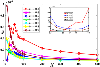
Figure 7. The locomotor efficiency of the composite plate.
Download figure:
Standard image High-resolution imageThe Froude efficiency discussed above only relates thrust to the total kinetic energy transmitted to the fluid, while the elastic potential energy stored in the flexible plate has been ignored. Here we want to investigate the efficiency of the external force used to drive its locomotion. In practice, the live fish or the bionic fish is driven by the muscle or servo actuator. It is supposed that the forces exerted on the junction point only. We can achieve the forces to maintain the motion of the composite plate as


In equations (32)–(34), the terms on the right side can be calculated at every moment. So we can achieve the work done by the external forces in a period as

We define a locomotor efficiency here, which represents the ratio of the kinetic energy to the work done by the external force

It is expected that the efficiency can give a more intuitive description on the energy cost of the locomotion of fish than Froude efficiency.
Figure 7 shows the locomotor efficiency of the composite plate. Due to the external forces do not exert on the nose of the live fish or bionic fish, the results of the onefold flexible plate are not included in the figure. It can be found that a lot of work is used to maintain the elastic deformation of the flexible plate and the locomotor efficiency has an order of 10−4, so the Froude efficiency maybe not enough to describe the efficiency of the locomotion of the composite plate. For l*= 0.3 ∼ 0.5, the locomotor efficiency first increases sharply then decreases with increasing stiffness, and finally tends to be stable. For l*= 0.6 ∼ 0.9, the locomotor efficiency decreases with increasing stiffness and finally tends to be stable. As the stiffness is small enough (K< 20), the locomotor efficiency increases with increasing l*. As the stiffness is large (K> 30), the locomotor efficiency first decreases sharply then increases slowly with increasing l*. The small figure at the up-right of figure 7 shows the tendency of the locomotor efficiency following l* at K = 10, 50, 100 and 500. The larger the stiffness is, the less variation of locomotor efficiency following l*. For small stiffness, K = 10, the locomotor efficiency increases following increasing l*. For large stiffness, K > 10, the locomotor efficiency first decreases and then increases following increasing l*.
From above discussion, we find that the tendency of the locomotor efficiency is very different from that of the Froude efficiency. So we think that it is necessary to analyze the locomotor efficiency to study the locomotion of fish thoroughly. As the stiffness is small, such as K = 10, larger flexible portion (l* = 0.9) results in larger locomotor efficiency. While the stiffness is large, such as K = 50, smaller flexible portion (l* = 0.3) gives a larger locomotor efficiency. This happens to coincide with the real swimming behavior of live fish, although the plate may be simple to model the whole fish body. In the nature, the fish with soft body, such as the eel and the larva of fish, often swim in anguilliform mode. While the fish with stiff body, such as Clupe and Scomber, often swim in carangiform mode.
5.2. The vibration of the flexible plate
The morphology response of the composite plate is an important issue for its self-propulsion. A thrust can be caused by the backward propagating wave on the composite plate, which drives the plate swim under the water. A 3D surface is constructed, where the axis x is the position on the plate. The axis y is the time, and the axis z is the deformation of the plate. It is expected that the evolution of the deformation of the plate can be demonstrated more clearly than the traditional envelope chart.
As that derived by Lighthill (1960) based on potential flow theory, the negative correlation between the gradient of the deformation at the tip  and the lateral velocity
  can leads to a negative propulsive velocity and Froude efficiency. The large amplitude and the small gradient of the deformation at the tip are beneficial to improve the propulsion of the plate. For all l* and K discussed in this paper, the correlation between
  and
and  is positive. The lateral amplitude and the gradient of the deformation at the tip affect the propulsive velocity and Froude efficiency simultaneously. For a specified l*, both the lateral amplitude and the deformation gradient of the tip decrease following the increasing stiffness K, as shown in figure 8. Due to the effect of the deformation gradient is predominant, so the propulsive velocity and the Froude efficiency increase with stiffness for arbitrary l*, as shown in figure 6. For a specified K, both the lateral amplitude and the deformation gradient of the tip decrease following the increasing stiffness l*, so the propulsive velocity and the Froude efficiency increase with stiffness for arbitrary K, as shown in figure 6.
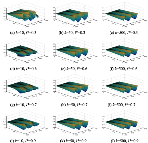
Figure 8. The evolution of the deformation of the plate.
Download figure:
Standard image High-resolution imageThe discussion in this section matches well with the result mentioned in Lighthill (1960), which proves the validity of the hydrodynamic study in this paper.
5.3. The forces on the plate
To investigate the effects of the rigid portion and the flexible portion on the locomotion of the composite plate, the average longitudinal hydrodynamic forces  distributed on the plate are shown in figure 9. The black dotted line represents the location of the junction. The left is the rigid portion, while the right is the flexible portion. The definition of
  is
is


Figure 9. The distributed hydrodynamic force on the plate.
Download figure:
Standard image High-resolution imagewhere,  is the longitudinal hydrodynamic forces distributed on the plate, N is the number of the data in integral multiple periods. To reduce the error, the data in eight periods are used in this paper.
An unexpected result is that the hydrodynamic force on the tail of the plate is positive for arbitrary l* and K, which is hindering the propulsion of the plate. Lighthill (1960) stated that the average thrust of the plate only rely on the motion of the tail point. So we conclude that the motion of the tail point plays a decisive role on the force distribution on the plate, rather than the thrust only produced at tail point. From figure 9(a), it can be found that the hydrodynamic force on the tail point is small as l*= 0.3 and K= 10. This may be the reason why most fish has a short ultra-soft membrane at the tail, which can reduce the resistance effectively. Although the positive values on the tail point of the flexible plate is large, but the range of its action is so small, whose effect on the resultant hydrodynamic force on the plate is limited.
The average thrust distribution on the rigid portion of the plate is smooth, while it fluctuates on the flexible portion. For small stiffness, such as K= 10 at l*= 0.3, the hydrodynamic force on the rigid portion is propelling the plate, while the force on the flexible portion is hindering the propulsion of the plate. For large stiffness, such as K> 50, the reverse is true. For other l*, the force on the rigid plate is hindering the propulsion, while the force on the flexible portion is fluctuating but repelling the plate overall as the stiffness is small (such as K= 10). As the stiffness is large enough, such as K> 50, the longitudinal force on whole composite plate varies gently with the location and repel the plate forward overall. The larger l* is, the greater the volatility of the force on the flexible plate is.
To investigate the significances of the pressure force and shear stress, figure 10 shows the distribution of the average pressure force and shear stress along the plate at K = 10. The pressure force on the plate is almost distributing uniformly for arbitrary l*. For l* = 0.3, the shear stress on the rigid plate is thrusting the plate forward, while the shear stress on the flexible plate is hindering the self-propulsion. For other l*, the shear stress on the rigid plate is hindering its propulsion, while the shear stress on the flexible plate is thrusting the plate.
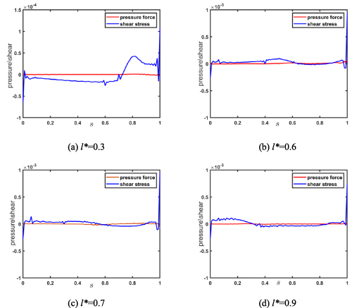
Figure 10. The distributed hydrodynamic force on the plate at K = 10.
Download figure:
Standard image High-resolution imageFigure 11 shows the external forces, see equations (32)–(34), exerted on the junction point to maintain the self-propulsion of the plate, the moment of force M is calculated by 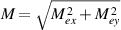 . For arbitrary l*, both the moment of force and the lateral force increase linearly following increasing stiffness K. For arbitrary stiffness, both the moment of force and the lateral force first increase from l* = 0.3 to l* = 0.8 then decrease from l* = 0.8 to l* = 0.9. These results echo the variation tendency of locomotor efficiency shown in figure 7. The flexible deformation of the plate needs large external force and energy to maintain, which reduces the energy utilization in the propulsion of the plate.

Figure 11. The external force exerted on the junction point. (a) The external moment of force. (b) The lateral force.
Download figure:
Standard image High-resolution image5.4. The flow structure around the plate
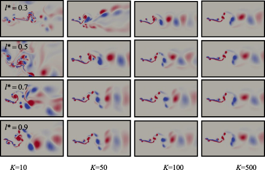
In this subsection, we want to investigate the flow structure around the composite plate, as shown in figure 12. The cases for four typical l* and four typical K are selected, and all vorticity contours shown here is grabbed as the rigid plate reaches its lowest location.
Figure 12. The vorticity contour around the plate: the rows from top to bottom are l* = 0.3, 0.5, 0.7 and 0.9, respectively; the columns from left to right are K = 10, 50, 100 and 500, respectively.
Download figure:
Standard image High-resolution image
For all cases, the reverse Karman vortices can be observed in the wake of the plate, which is emblematic for the locomotion of the fish. The larger the stiffness is, the smaller the difference between the vortex contours at different l*. Although the lateral motion of the head point is confined, the vortices pair shedding from it can also be observed. In most cases, except l*= 0.3, 0.5 and K= 10, the vortices pair can merge into the vortices shedding from the tail.
As l* and K are both small, such as l*= 0.3, 0.5 and K= 10, the vortices around the plate is tanglesome. The vortices shedding from both the head and tail point of the plate deposit in a limited region due to the low propulsive velocity of the plate. These vortices interact with each other drastically, which induces the unsteady motion, as the IM state shown in Hua et al (2013). The tail of the plate is so soft that the strength of the vortex can curl it, for example in l*= 0.3 and K= 10, which cause a positive (hindering) force on the flexible plate, see figure 9(a). As l*= 0.3 and K= 50, the wake behind the plate is asymmetry, this is due to the inequality of the propulsive velocity during different half period (Hua et al 2013). For other cases, 2P mode vortex shedding mode from the tail can be observed. Due to the participation of the vortex shedding from the head, 2T vortices can be seen in the wake very close to the tail.
6. Conclusions
In this paper, the self-propulsion of the rigid-flexible composite plate was simulated numerically. The ratio between the length of the flexible portion and the rigid portion and the stiffness of the flexible portion were varied to study their effect on the propulsion. The pitch motion of the rigid plate was given, and the composite plate was supposed to be driven by the forces exerted on the junction point. By this unique modeling approach, we have achieved some conclusions.
- (a)The tendencies of the propulsive velocity and the Froude efficiency of the composite plate following stiffness are similar to those of the onefold flexible plate. The stiffer the flexible plate is, the larger Froude efficiency achieves. And the larger proportion of the flexible plate, the larger Froude efficiency and propulsive velocity of the composite plate.
- (b)A locomotor efficiency is proposed here, which involves the elastic potential energy stored in the flexible plate. It is found that the case with larger flexible portion is efficient for the ultra-soft plate, while the case with smaller flexible portion is efficient for the stiff plate. These results happen to coincide with the swimming behavior of live fish.
- (c)We find that the hydrodynamic force at the tail is hindering the propulsion of the plate, which may be not consistent with the assumption of previous research. So we conclude that the motion of the tail point plays a decisive role on the force distribution on the plate, rather than the thrust only produced at tail point. From this conclusion, we think that the short ultra-soft membrane at the tail of the real fish is an important feature to improve its swimming behavior.
Acknowledgments
The authors are grateful to the support from the National Natural Science Foundation of China (Grant No. 11802063).