


Abstract
In the statistical steady state of forced-dissipative turbulence governed by the 2D incompressible Navier–Stokes (NS) equation, the difference between the energy flux ΠE(k) and the enstrophy flux ΠZ(k), k2ΠE(k) − ΠZ(k), where k is the wavenumber, has been proved to be negative outside the forcing wavenumber range. This is often referred to as the Danilov inequality and is important for determining the directions of the energy and enstrophy fluxes in the inertial ranges for 2D NS turbulence. We investigate numerically whether or not this inequality holds for two-layer quasi-geostrophic (QG) potential vorticity equations, which are a generalization of the vorticity equation for the 2D NS system. In two-layer QG systems forced by a horizontally homogeneous, baroclinically unstable basic flow, the corresponding difference between the total energy and total potential enstrophy fluxes is mathematically sign-indefinite due to the presence of the internal forcing term. Moreover, even if we concentrate on outside of the internal forcing range, the flux difference is still sign-indefinite when the dissipation mechanisms are asymmetric between the upper and lower layers. However, in our numerical experiments adopting both the internal forcing and asymmetric dissipations, the flux difference is negative across the whole wavenumber range. That is, the Danilov inequality continues to hold for two-layer QG systems, even though this cannot be proved mathematically.
Export citation and abstract BibTeX RIS
Communicated by Peter Haynes
1. Introduction
The quasi-geostrophic (QG) potential vorticity equation is one of the models used to describe large-scale atmospheric and oceanic circulations on the Earth and has a similar form to the vorticity equation derived from the 2D incompressible Navier–Stokes (NS) equation. Thus, turbulence governed by the QG potential vorticity equation, called geostrophic turbulence, is regarded as a generalization of 2D NS turbulence and has been studied from physical and geophysical perspectives.
It is well known that two inertial ranges, namely, the energy and enstrophy inertial ranges, coexist in the statistical steady state of 2D NS turbulence, forced in a narrow wavenumber range (Kraichnan 1967, Leith 1968, Batchelor 1969). The energy inertial range is formed at wavenumbers below the forcing wavenumber range. In the energy inertial range, the energy spectrum is proportional to k−5/3, where k stands for the wavenumber, and the energy is transferred from the forcing wavenumber range towards lower wavenumbers. In contrast, the enstrophy inertial range is formed at wavenumbers above the forcing wavenumber range. In the enstrophy inertial range, the energy spectrum is proportional to k−3, and the enstrophy is transferred from the forcing wavenumber range towards higher wavenumbers. These properties are attributed to the existence of two inviscid invariants, kinetic energy and enstrophy.
Since the QG potential vorticity equation also has two inviscid invariants, total energy and total potential enstrophy, it was believed that the wavenumber dynamics of geostrophic turbulence would resemble that of 2D NS turbulence. However, when Tung and Orlando (2003) (hereinafter TO03) conducted numerical simulations of two-layer QG potential vorticity equations, the simplest QG potential vorticity equations capable of density stratification and baroclinicity, they found a curious energy spectrum that was different to the inertial range spectrum for 2D NS turbulence. Their total energy spectrum was proportional to k−3 above the forcing wavenumber range, changing to k−5/3 as the wavenumber increased further, and they proposed a mechanism to explain this transition. Their spectrum resembled an atmospheric energy spectrum, the so-called Nastrom–Gage (NG) spectrum. As a result, their work is interesting from the viewpoint of both 2D NS turbulence and its geophysical applications.
The NG spectrum is considered to be a universal property of atmospheric circulation at high and middle altitudes on the Earth. Originally, Nastrom and Gage (1985) found that the energy spectra of zonal and meridional winds and of the temperature near the tropopause obtained from aircraft measurements were proportional to k−3 between wavelengths of a few thousand and a few hundred kilometers. Furthermore, they found that the relationships changed to k−5/3 at smaller scales below a hundred kilometers. The existence of the NG spectrum has been confirmed by spherical harmonic analysis of both simulation results of general circulation models and other observational data (Koshyk and Hamilton 2001, Burgess et al 2013). Then, the wavenumber k should be interpreted as the spherical harmonic wavenumber. In particular, much work has been done in an attempt to understand how the NG spectrum is formed from the viewpoint of both 2D NS turbulence and geostrophic turbulence.
The NG spectrum's k−3 region is regarded as being analogous to the enstrophy inertial range spectrum of forced-dissipative 2D NS turbulence (Lindborg 1999), but the formation of the k−5/3 region has been shown to be dominated by internal gravity waves (e.g. Koshyk and Hamilton 2001, Hamilton et al 2008, Callies et al 2014). In contrast, TO03 were able to reproduce an NG-like spectrum by numerically simulating a two-layer QG model with the gravity waves filtered out.
The mechanism proposed by TO03 for the formation of the k−5/3 region in the two-layer QG potential vorticity equations (the TO mechanism from now on) is as follows. Both the total energy and total potential enstrophy injected around the internal deformation radius due to baroclinic instability are transferred towards higher wavenumbers. The total potential enstrophy inertial range is formed at wavenumbers where the total energy flux is less efficient than the total potential enstrophy flux, and the total energy inertial range is formed at wavenumbers where the total energy flux is more efficient than the total potential enstrophy flux. TO03 called the total energy transfer towards higher wavenumbers the hidden energy cascade, since such a property is as yet unknown in 2D NS turbulence in the high Reynolds number limit.
TO03 introduced the following flux difference to express the extent to which the total energy flux dominates the total potential enstrophy flux:

Here, ΠE(k) is the total energy flux, namely, the total energy transferred from lower to higher wavenumbers across wavenumber k per unit time. ΠZ(k) is the total potential enstrophy flux, defined similarly. The TO mechanism implies that the k−5/3 spectrum is formed in the wavenumber range where

In contrast, for the statistical steady state of 2D NS turbulence, forced in a narrow wavenumber range, the inequality

has been proved mathematically for all k outside the forcing wavenumber range (Gkioulekas and Tung 2007). Here, ΠE(k) and ΠZ(k) should be interpreted as the kinetic energy and enstrophy fluxes, respectively. This is often referred to as the Danilov inequality4 and even holds for the two-layer QG model if dissipation processes, such as the Ekman friction due to the presence of boundaries and viscosity acting at small scales, are symmetric between the upper and lower layers and k is assumed to be outside the forcing wavenumbers (Gkioulekas 2014). However, the sign of the flux difference in (1) is not well defined when the asymmetric dissipation processes and an internal forcing due to a baroclinically unstable basic flow are involved (Gkioulekas 2014). In fact, TO03 introduced an asymmetric Ekman friction term and an internal forcing due to a baroclinically unstable basic flow in their model, even though they assumed that the viscosities were symmetric.
As mentioned above, the TO mechanism is interesting for both generalizing 2D NS turbulence and its geophysical applications, but its validity has been questioned (Smith 2004, Tung 2004). Interestingly, there have been no numerical simulations of the two-layer QG potential vorticity equations that reproduce the k−5/3 spectrum, except for those by TO03. Moreover, the Danilov inequality for the two-layer QG model has not been investigated numerically yet, although sufficient conditions for which the inequality is violated have been theoretically investigated by Gkioulekas (2012, 2014).
Although TO03 stated that the total energy flux towards larger wavenumbers, which is referred to as the downward total energy flux, is crucial for explaining the k−5/3 spectrum, the existence of such a flux would not be at all surprising. Since all numerical simulations of 2D or geostrophic turbulence have been performed at high but finite Reynolds numbers, such a downward energy flux must exist to balance the energy transferred towards larger wavenumbers with the energy dissipated at the dissipation scale. This issue has already been highlighted by Smith (2004). In this sense, the violation of the Danilov inequality is highly significant for the formation of the k−5/3 spectrum in geostrophic turbulence. Motivated by this, we investigate the Danilov inequality by simulating the two-layer QG potential vorticity equations numerically. Although Gkioulekas (2012) studied the Danilov inequality for two-layer geostrophic turbulence excited by externally prescribed forcing, this paper discusses the Danilov inequality for the system excited by an internal forcing due to a baroclinically unstable mean flow. This is a case that Gkioulekas (2012) left as an unsolved problem. Furthermore, as will be explained later, we adopt asymmetric dissipations, which are the potential causes for which the Danilov inequality is violated as pointed out by Gkioulekas (2014), to the system studied here. In this sense, the present study is considered as being the numerical investigation of the problem studied by Gkioulekas (2014) theoretically.
The picture of the wavenumber dynamics of two-layer geostrophic turbulence is summarized in Vallis (2006). Most geostrophic turbulence studies have mainly focused on the wavenumber range k ≲ kd up to now, where kd stands for the inverse of the deformation radius. In contrast, the dynamics in the range k ≳ kd of geostrophic turbulence has not attracted researcher interest, because it has been considered to be the same as with dynamics of 2D NS turbulence. However, the wavenumber range k ≳ kd where the TO mechanism might emerge is our region of interest.
The remainder of this paper is organized as follows. In section 2, we introduce the model and present the corresponding QG potential vorticity equations. In section 3, we discuss the Danilov inequality for this system and discuss its importance for 2D NS turbulence. In section 4, we simulate the two-layer QG potential vorticity equations numerically and examine whether or not the Danilov inequality holds. Finally, in section 5, we present a brief discussion and our conclusions.
2. Model
2.1. Governing equations
We consider a Boussinesq fluid consisting of two immiscible layers of equal depth on an f-plane and confined between rigid horizontal plates. We assume that the fluid's motion is nearly geostrophic. This means that the fluid's governing equations are the following QG potential vorticity equations:

where, the subscripts 1 and 2 refer to the upper and lower layers, respectively, and  and
and  are the potential vorticity and stream function, respectively, of the jth layer (see e.g. Vallis 2006). In addition,
  is the horizontal Jacobian, and δij is the Kronecker delta. The flow domain
  is assumed to be a rectangle of size Lx × Ly. In addition, we assume the presence of dissipation processes: the second term on the right-hand side of (4) represents the hyper-viscosity of order γ, and the third term is the Ekman friction term, which represents the damping of the lower layer's relative vorticity by the lower boundary. νj is the hyper-viscosity coefficient for the jth layer and κ is the Ekman friction coefficient. The fourth term represents the Newtonian temperature damping due to radiative cooling towards the prescribed basic states
  , and α represents the Newtonian cooling coefficient. In addition, the x and y directions are considered to be eastwards and northwards, respectively, for geophysical cases.
We assume that the basic states are horizontally uniform steady flows with a vertical shear:

where the positive constant U represents the magnitude of velocities for the upper and lower layers. From the thermal wind balance (Vallis 2006), the presence of basic states with a vertical shear given by (6) implies that there is a temperature difference along the y direction.
We decompose the stream functions into basic state and perturbation components, as follows:

where primed quantities represent perturbation and unknown variables. In addition, we introduce the barotropic and baroclinic stream functions, ψ and τ, as follows:


Then, the governing equations (4) become


where qψ and qτ are the barotropic and baroclinic potential vorticities, respectively. Here, we have introduced the notation ν ≡ ν1 and Δν ≡ ν2 − ν1. To simplify both the numerical simulations and theoretical discussions, we adopt doubly periodic boundary conditions for both ψ and τ. These are the fundamental equations considered in this study.
Models similar to (10) and (11) have been used in studies of geostrophic turbulence by many researchers (see e.g. Salmon 1978, 1980, Haidvogel and Held 1980, Larichev and Held 1995, Tung and Orlando 2003, Arbic and Flierl 2004, Thompson and Young 2006, Gkioulekas 2012, 2014) and it is thus a very standard model for geostrophic turbulence studies. One of the notable characteristics of our model is the presence of an asymmetric hyper-viscosity term. The hyper-viscosity has been considered as a useful computational tool for numerical simulations to mimic sub-grid scale dissipations. There are no physical reasons for the asymmetry of the hyper-viscosity. Thus, previous studies have generally set the viscosity coefficients ν1 and ν2 to be of equal value. However, Gkioulekas (2014) discussed the effect of the asymmetric hyper-viscosity on the Danilov inequality and indicated that the Danilov inequality might be violated due to the presence of the asymmetric hyper-viscosity. To consider this possibility, we adopt the asymmetric hyper-viscosity in our model. Another characteristic of our model is that we neglect the β effect, which represents the dependence of the reference frame's rotation on the y coordinate or that on the Earth's curvature. As stated in section 1, the main purpose of the present study is to investigate the unsolved problem in Gkioulekas (2012, 2014). Thus, we follow the setting up of the problem of his studies, in which the Danilov inequality on an f-plane was investigated. The β effect does not directly affect the sign of (1) because it does not arise explicitly in the evolution equations for the total energy and total potential enstrophy spectra. In addition, the impact of the β effect on the NG spectrum's k−5/3 region would be negligible, since the so-called Rhines scale (Rhines 1975) is much larger than the wavenumber range of the k−5/3 spectrum. Therefore, similar to Gkioulekas (2012, 2014), we neglect the β effect in the present study.
2.2. Modal total energy and total potential enstrophy equations
Since we have adopted the doubly periodic boundary conditions, we can expand the stream functions, ψ and τ, as Fourier series:


where  and nx and ny are integers. The summation
  is taken over all of the integer vectors (nx, ny). The evolution equation for the modal total energy is then as follows:


Here,  and
and  are the transfer function, forcing term and dissipation term for the modal total energy equation, respectively. The derivation of (16)–(20) is summarized in appendix A. The terms that make up (18) are given by (A.4)–(A.7) and (A.9)–(A.14). If we sum (16) over all wavenumber vectors, the term
  , which arises from the governing equations' nonlinear terms, vanishes because the total energy is an inviscid invariant. The sign of
  is indefinite, but this is the system's only energy source, so we expect
  to be positive if we sum it over all wavenumber vectors and average the result over some interval. If
  is negative definite. The sign of the asymmetric hyper-viscosity term in the modal total energy equation, which is proportional to Δν in (20), is indefinite. In contrast, the Ekman friction and Newtonian cooling terms (the terms proportional to κ and α, respectively, in (20)) are both negative definite.
In addition, the evolution equation for the modal total potential enstrophy can be obtained similarly:


Here,  and
and  are the transfer function, forcing term and dissipation term for the modal total potential enstrophy equation, respectively. The ratio of the forcing terms for the modal total potential enstrophy and modal total energy,
  , is exactly
  . Unlike for the modal total energy equation, here the sign of the asymmetric hyper-viscosity term is definite and the sign of the Ekman friction term is indefinite. As we will show later, the fact that the signs of the asymmetric hyper-viscosity term for the modal total energy equation and Ekman friction term for the modal total potential enstrophy equation are not definite is one of the potential causes of the Danilov inequality violation in this system.
3. Danilov inequality
As in the studies by Gkioulekas and Tung (2007) and Gkioulekas (2012, 2014), we now discuss this system's flux inequality. To simplify the discussion, we extend the flow domain to be infinite and express the stream functions, ψ and τ, in terms of their Fourier transforms. Taking the angle average of (16) in wavenumber space and taking the ensemble average of the resulting equation leads to the following evolution equation for the total energy spectrum:


Here, E(k) is the total energy spectrum, ΠE(k) is the total energy flux and FE(k) and DE(k) are the total energy forcing and total energy dissipation spectra, respectively. Here, the angle brackets denote the angle average in wavenumber space and ensemble average, as appropriate. The following evolution equation for the total potential enstrophy spectrum can similarly be obtained from (21)–(25):


Here, Z(k) is the total potential enstrophy spectrum, ΠZ(k) is the total potential enstrophy flux and FZ(k) and DZ(k) are the total potential enstrophy forcing and total potential enstrophy dissipation spectra, respectively.
If we assume a statistical steady state and integrate both (26) and (31) with respect to wavenumber from k to infinity, we obtain


where we have used the total energy and total potential enstrophy conservation laws,  and
and  . In addition, subtracting (37) from (36) multiplied by k2 yields

By substituting (19), (20), (24), (25), (29), (30), (34) and (35) into the integrand of (38), we obtain the following equation:
We cannot determine the sign of both ![${\mathfrak{Re}}[\hat{\psi }({\boldsymbol{k}}){\hat{\tau }}^{* }({\boldsymbol{k}})]$](https://content.cld.iop.org/journals/1873-7005/51/5/055507/revision2/fdrab2eadieqn20.gif) and
and ![${\mathfrak{Im}}[\hat{\psi }({\boldsymbol{k}}){\hat{\tau }}^{* }({\boldsymbol{k}})]$](https://content.cld.iop.org/journals/1873-7005/51/5/055507/revision2/fdrab2eadieqn21.gif) , so the forcing, asymmetric hyper-viscosity and Ekman friction terms all contribute to the sign of the flux difference being indefinite.
, so the forcing, asymmetric hyper-viscosity and Ekman friction terms all contribute to the sign of the flux difference being indefinite.
We note in passing that the integral in (39) can be changed from  to
to  , but the integrand remains unchanged. This form of the flux difference is obtained when the total energy and total potential enstrophy fluxes are derived by integrating (26) and (31) with respect to wavenumbers from 0 to k, respectively, and using the conservation laws,
  and
and  .
.
If we set Δν = 0, κ = 0 and  , (39) reduces to the Danilov inequality for the 2D NS system. Here, we note that the forcing wavenumbers should be interpreted as being outside the integration interval. Since
  in the interval
  , the flux difference is negative definite. As noted above, the integral interval in (39) can be changed from
  to
to  . This leaves the sign of the flux difference unchanged, since
  in the interval
  , so the flux difference is negative definite for wavenumbers both above and below the forcing wavenumbers for the 2D NS system. This is the Danilov inequality for the 2D NS system. It is well known that the enstrophy flux is zero in the
  spectral range for 2D NS turbulence in the high Reynolds number limit (Kraichnan 1967). In conjunction with the Danilov inequality, this means that the energy flux is negative in the k−5/3 spectral range, i.e. the energy is being transferred to lower wavenumbers. It is also well known that the energy flux is similarly zero in the k−3 spectral range for 2D NS turbulence in the high Reynolds number limit, which, in conjunction with the Danilov inequality, means that the enstrophy flux is positive in the k−3 spectral range, i.e. the enstrophy is being transferred to higher wavenumbers. These properties can be derived without assuming any closure approximations, so the Danilov inequality is significant for the 2D NS system.
4. Numerical simulations
4.1. Overview
In this section, we conduct direct numerical simulations of turbulence governed by (10) and (11). First, we outline the numerical method, initial conditions and calculation resolution. The values used for the parameters in (10) and (11) were essentially the same as those used in Larichev and Held (1995) and Arbic and Flierl (2004) (hereinafter LH95 and AF04, respectively).
The pseudo-spectral method was used with double-precision arithmetic at a resolution of N2 (the number of grid points in the square computational domain [0, L] × [0, L]), and the truncation wavenumber kT was chosen according to the two-thirds dealiasing rule. The domain size was L = 2π. Time integration was performed using the Runge–Kutta–Gill scheme with a fixed time step Δt, ensuring that Δt values used satisfied the Courant–Friedrichs–Lewy condition.
The initial conditions were set by generating uniform random numbers in the interval [0, 2π] for the phases of  and
and  . The initial amplitudes of
  and
and  were normalized so that the barotropic and baroclinic energy spectra, Eψ(k) and Eτ(k), were independent of k:
First, the system was spun up at a resolution of N = 256 until t = t1, and then, numerical integration was performed at a higher resolution of N = 512 until t = t2. The results of the higher resolution calculations were analyzed and averaged over the interval between  and t2 to improve the statistical convergence of the results. Since, as shown in the previous section, the Newtonian damping term in (11) does not contribute to violating the Danilov inequality, it is omitted in the following discussion, i.e. α = 0.
Scaling the spatial coordinates by  , the time by
  , the stream functions by
  and the potential vorticities by
  leads to the governing equations being controlled by the following three dimensionless parameters:

The parameter  , which Arbic and Flierl (2003) call the throughput, is particularly significant because it controls the partition of the total energy into barotropic and baroclinic components or into kinetic energy and available potential energy. For example, when the throughput is small, the total energy is dominated by the available potential energy and the system behaves as if it is equivalent barotropic. In contrast, when the throughput is large, the total energy is dominated by the kinetic energy and the system behaves as if it is barotropic.
To resolve the high-wavenumber dynamics in the k > kd region, our region of interest, and ensure that there is sufficient spectral room for the upward energy cascade in k < kd, the region of primary interest for most geostrophic turbulence studies, we set kd = 10 for all simulations, even though LH95 used kd = 50 for their kT = 128 resolution simulations. In addition, we fixed U = 2.5 × 10⁻², making our Ukd value equivalent to that used in LH95. By changing the value of κ, we could vary the throughput from 1.25 × 10⁻² to 25, an equivalent range to that studied in AF04. Note in passing that we could not obtain from numerical simulations the statistical steady state of the system when we adopted  . Since these experiments are those for changing the throughput value, we shall refer to these as the TH experiments. Note that the estimated throughput in the TO03 experiments was nearly 27.3 (see appendix B).
The hyper-viscosity parameters used in the present study were similar to those used in LH95. They used γ = 4 and ν = 5.12 × 10⁻¹⁶ for kT = 128 resolution simulations. We decided to maintain the e-folding time for the hyper-viscosity at the truncation wavenumber at the value used in LH95, so we set ν = 5.12 × 10−16 × (128/kT)2γ. The numerical parameters used in the TH experiments are summarized in table 1.
Table 1. Parameters used for the TH experiments.
| Experiment | κ | 2Ukd/κ | t1 | t2 | tave | Δt | Δν |
|---|---|---|---|---|---|---|---|
| TH1 | 0.02 | 25 | 1000 | 1500 | 200 | 6.25 · 10−4 | 0 |
| TH2 | 0.04 | 12.5 | 1000 | 1500 | 200 | 6.25 · 10−4 | 0 |
| TH3 | 0.08 | 6.25 | 1000 | 1500 | 200 | 6.25 · 10−4 | 0 |
| TH4 | 0.16 | 3.125 | 1000 | 1500 | 200 | 6.25 · 10−4 | 0 |
| TH5 | 0.4 | 1.25 | 1000 | 1500 | 200 | 6.25 · 10−4 | 0 |
| TH6 | 0.8 | 0.625 | 1000 | 1500 | 200 | 6.25 · 10−4 | 0 |
| TH7 | 2 | 0.25 | 1000 | 1500 | 200 | 6.25 · 10−4 | 0 |
| TH8 | 8 | 6.25 · 10−2 | 10000 | 10500 | 200 | 6.25 · 10−4 | 0 |
| TH9 | 40 | 1.25 · 10−2 | 64000 | 66000 | 500 | 1.25 · 10−3 | 0 |
We made sure to resolve the dissipation ranges for the total energy and total potential enstrophy spectra, because this affects the accuracy of the inertial range statistics (see e.g. Smith 2004, Watanabe and Gotoh 2007). If the viscosity coefficients  and ν2 are not large enough to remove the total energy and total potential enstrophy transferred to higher wavenumbers, their spectra will exhibit transitions to shallower slopes near the truncation wavenumber. One of our criteria for resolving the dissipation ranges is that the dissipation wavenumbers have to be smaller than the truncation wavenumber kT. By dimensional analysis, the dissipation wavenumber kε, which is based on the rate of total energy dissipation due to hyper-viscosity (εν) and is known as the energy dissipation wavenumber, can be defined as


Here,  indicates the spatial average of a given quantity A, and
  is the average viscosity coefficient, i.e.
  . The enstrophy dissipation wavenumber kη, which is similarly based on the rate of total potential enstrophy dissipation due to hyper-viscosity (ην), can be defined as


Here, table 2 gives the values of εν, ην, the rates of total energy and total potential enstrophy dissipations due to Ekman friction, εκ and ηκ, where εκ and ηκ are defined as


These results show that the bulk of the total energy is dissipated due to Ekman friction, independent of the throughput. In contrast, hyper-viscosity is the main cause of potential enstrophy dissipation for high throughputs, but as the throughput decreases, the contributions of hyper-viscosity and Ekman friction become broadly equal. From the evolution equations of the potential enstrophy in the individual layers, the potential enstrophies in the individual layers are inviscid invariants. However, the present system is forced by the baroclinic instability of basic flow. Then, the same amount of potential enstrophy,  , is supplied to the individual layers. We can interpret these results in terms of the energy and potential enstrophy balances in the individual layers. Since the viscosity is the only dissipation mechanism of the potential enstrophy in the upper layer, the potential enstrophy in the upper layer is dissipated by the hyper-viscosity, independent of the throughput. In contrast, the Ekman friction and hyper-viscosity are the dissipation mechanisms in the lower layer. Then, the potential enstrophy in the lower layer is mainly dissipated by the hyper-viscosity for high throughputs. As the throughput decreases, the Ekman friction tends to dominate more and more. In the case of the lowest throughput realized in the present simulations, the potential enstrophy in the lower layer is mainly dissipated by the Ekman friction. In contrast, the upper layer energy is transferred to the lower layer and the upper and lower layers' energies are dissipated by the Ekman friction, independent of the throughput.
Table 2. Results of the TH experiments. Here, εκ and εν are the rates of total energy dissipation due to Ekman friction and hyper-viscosity, respectively. ηκ and ην are the corresponding potential enstrophy dissipation rates, and E is the total energy.
| Experiment | εκ | εν | ηκ | ην | E |
|---|---|---|---|---|---|
| TH1 | 0.479 906 · 10−1 | 0.238 492 · 10−3 | 0.247 644 | 0.379 799 · 101 | 0.268 957 · 101 |
| TH2 | 0.757 129 · 10−1 | 0.414 733 · 10−3 | 0.832 560 | 0.649 352 · 101 | 0.231 900 · 101 |
| TH3 | 0.167 871 · 10−1 | 0.899 281 · 10−4 | 0.463 903 | 0.123 716 · 101 | 0.377 302 |
| TH4 | 0.272 875 · 10−2 | 0.123 826 · 10−4 | 0.124 204 | 0.148 625 | 0.596 710 · 10−1 |
| TH5 | 0.592 001 · 10−3 | 0.281 146 · 10−5 | 0.295 460 · 10−1 | 0.301 525 · 10−1 | 0.131 926 · 10−1 |
| TH6 | 0.341 400 · 10−3 | 0.167 693 · 10−5 | 0.170 332 · 10−1 | 0.173 624 · 10−1 | 0.113 376 · 10−1 |
| TH7 | 0.237 437 · 10−3 | 0.119 873 · 10−5 | 0.119 630 · 10−1 | 0.119 538 · 10−1 | 0.185 097 · 10−1 |
| TH8 | 0.142 245 · 10−3 | 0.745 009 · 10−6 | 0.710 402 · 10−2 | 0.724 520 · 10−2 | 0.563 060 · 10−1 |
| TH9 | 0.328 415 · 10−4 | 0.208 469 · 10−6 | 0.151 022 · 10−2 | 0.188 764 · 10−2 | 0.648 866 · 10−1 |
Figure 1 shows how the energy and enstrophy dissipation wavenumbers depend on the throughput, indicating that both dissipation wavenumbers are less than the truncation wavenumber kT = 170.

Figure 1. Dependence of the energy dissipation wavenumber kε, enstrophy dissipation wavenumber kη and transition wavenumber ktrans on the throughput.
Download figure:
Standard image High-resolution imageAnother criterion for measuring the dissipation range is that of the spectrum of total energy dissipation due to hyper-viscosity, which is defined by
which decays sufficiently rapidly in the wavenumber range kε ≲ k < kT. Figure 2 shows the dissipation spectra for four selected experiments, TH2, TH5, TH7 and TH9. Here, the dissipation spectra take their maximum values around kε and then decay rapidly as the wavenumber increases further. Although we have only shown the dissipation spectra for some of the experiments, the dissipation spectra for the other TH experiments behave similarly. We can thus conclude that our experiments resolve the dissipation range well.

Figure 2. Dissipation spectra for experiments TH2, TH5, TH7 and TH9. Abscissa is normalized by the energy dissipation wavenumber kε, and the ordinate is normalized by kε and the rate of total energy dissipation due to hyper-viscosity εν.
Download figure:
Standard image High-resolution imageThis study focuses on the energy and enstrophy transfers in wavenumber space. To ensure the validity of our numerical simulations and analysis, we also verified that the transfer functions that make up (18) satisfy conservation laws, and this is discussed in appendix C.
Figure 3 shows snapshots of the barotropic and baroclinic potential vorticities for the same four TH experiments as in figure 2. As the throughput decreases, the barotropic potential vorticity fields change drastically from circular to more ribbon-like shapes, while the baroclinic potential vorticity fields change from circular to more blob-like shapes. On the other hand, the kinetic and available potential energy fields have circular structures for large throughputs, but become ribbon-shaped (surrounding the available potential energy extrema) and blob-shaped, respectively, as the throughput decreases, as pointed out by AF04 (figures are not shown). In addition, the structures of the barotropic and baroclinic stream functions become similar as the throughput decreases (figures are not shown ). Since the lower layer's stream function is ψ2 = ψ − τ, this indicates that its motion is reduced because of the bottom friction as the throughput decreases.
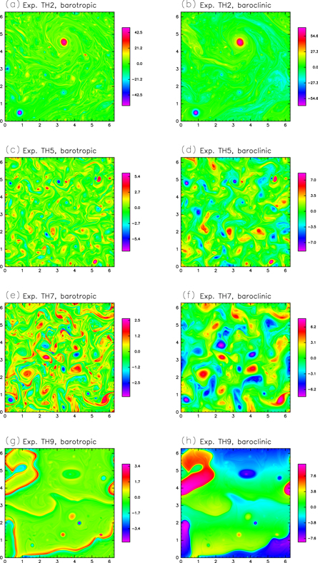
Figure 3. Barotropic (left) and baroclinic (right) potential vorticity fields at t = t2 for experiments TH2, TH5, TH7 and TH9.
Download figure:
Standard image High-resolution imageFigure 4 shows the dependence of the ratios of kinetic energy K to total energy E and barotropic energy Eψ to total energy E on the throughput. Here, K, Eψ and E are defined by


Note that the difference between Eψ/E and K/E is equal to Kτ/E, where Kτ is the baroclinic kinetic energy. The potential energy dominates for small throughputs, but the kinetic energy increases with throughput. In addition, the kinetic energy is dominated by the barotropic component for large throughputs. Taken together, those results indicate that our numerical experiments cover a wide range of two-layer geostrophic turbulence dynamics.
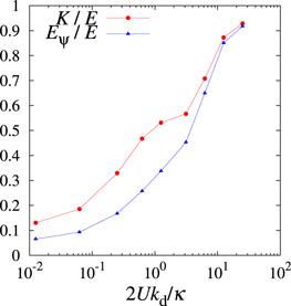
Figure 4. Dependence of the ratios of kinetic energy to total energy, K/E, and barotropic energy to total energy, Eψ/E, on the throughput.
Download figure:
Standard image High-resolution image4.2. Danilov inequality
Although this paper's main aim is to examine whether or not the Danilov inequality holds for two-layer geostrophic turbulence, in this section we shall also investigate fundamental turbulence properties such as the total energy spectrum, total energy and total potential enstrophy fluxes. First, figure 5 gives the total energy spectra for all of the TH experiments, showing that they follow a power law of the form E(k) ∼ k−δ with 3 ≲ δ ≲ 4 in the wavenumber range kd ≲ k ≲ kε and smoothly decay as k increases further. Note that there is no transition from E(k) ∼ k−δ to E(k) ∼ k−5/3. The exponent δ is close to 3 for larger throughputs and increases as the throughput decreases. The exponents are very close to those of the enstrophy inertial range spectra for forced-dissipative 2D NS turbulence.
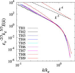
Figure 5. Total energy spectra for all TH experiments. Abscissa is normalized by the dissipation wavenumber kε, and the ordinate is normalized by kε and the energy dissipation rate εν. Only the wavenumber range k > kd is shown.
Download figure:
Standard image High-resolution imageNow, we develop this analysis of the total energy spectra further. TO03 defined the transition wavenumber ktrans as

They stated that the enstrophy inertial range occurs in the wavenumber range k < ktrans and the energy inertial range appears in the wavenumber range k > ktrans. Using (42) and (44), the transition wavenumber is related to the dissipation wavenumbers via

For the energy inertial range to exist, the transition wavenumber ktrans must be less than the energy dissipation wavenumber kε and (53) indicates that the transition wavenumber is less than the energy dissipation wavenumber if kε > kη. However, figure 1 shows that kη was very similar to but slightly larger than kε in all of the TH experiments, which means that the energy inertial range was not present in these experiments. This is consistent with the total energy spectrum analysis. Note that it is impossible to control the values of kε and kη a priori, since our model is internally forced by an unstable basic flow. Furthermore, as shown in the previous subsection, our numerical experiments cover a wide regime of two-layer geostrophic turbulence dynamics. Thus, the relation kε < kη obtained by the numerical simulations should be interpreted as one of the intrinsic properties of the present system.
Next, we examine the total potential enstrophy and total energy fluxes, which are shown in figure 6, normalized by their dissipation rates due to hyper-viscosity. Again, results are only presented for four TH experiments, but the results of all of the TH experiments were analyzed. In addition, these figures only show the fluxes in the range k > kd, since this is our wavenumber range of interest. The total potential enstrophy flux, which is equal to the total potential enstrophy dissipation rate ην, exists over a wide range of wavenumbers less than kε. Likewise, the total energy flux, which is equal to the total energy dissipation rate εν, is present over a similar but narrower wavenumber range. In this sense, there is the so-called hidden energy cascade, as suggested by TO03. We note in passing that the fluxes in the range k ≲ kd are consistent with classical theories of two-layer geostrophic turbulence, as shown in figure 2 of Thompson and Young (2006).
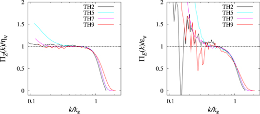
Figure 6. Total potential enstrophy (left) and total energy (right) fluxes for experiments TH2, TH5, TH7 and TH9. Abscissas are normalized by the energy dissipation wavenumber kε. Ordinates for the potential enstrophy fluxes and total energy fluxes are normalized by the total potential enstrophy dissipation rate ην and the total energy dissipation rate εν, respectively. Only the wavenumber range k > kd is shown.
Download figure:
Standard image High-resolution imageFinally, we examine whether or not the Danilov inequality holds by computing the flux difference (1) and considering their sign. Figure 7 shows that the flux difference is negative over the whole wavenumber range 1 ≤ k ≤ kT and this was confirmed by checking the numerical flux difference values. Thus, the Danilov inequality held in these experiments. As shown in (39), functional forms of the forcing spectra FE(k) and FZ(k) are key factors in determining the sign of the flux difference. The numerical results show that those spectra are significantly distributed in the range k ≤ kd and are mainly positive there. (figures are not shown.) Moreover, the relation  is held in the same wavenumber range, since
  . As a result, the forcing spectra make the flux difference positive there, as shown in figure 8, which shows the contributions of the forcing spectra on the flux difference,
 ![${\left[{k}^{2}{{\rm{\Pi }}}_{E}(k)-{{\rm{\Pi }}}_{Z}(k)\right]}_{{\rm{forc}}}\equiv -{\int }_{k}\infty \left[{k}^{2}{F}_{E}({k}^{{\rm{{\prime} }}})-{F}_{Z}({k}^{{\rm{{\prime} }}})\right]\,{\rm{d}}{k}^{{\rm{{\prime} }}}$](https://content.cld.iop.org/journals/1873-7005/51/5/055507/revision2/fdrab2eadieqn52.gif) . In contrast, the dissipation spectra due to the Ekman friction are significant in the same wavenumber range, compensate the contribution of the forcing spectra on the flux difference and make the flux difference negative.
. In contrast, the dissipation spectra due to the Ekman friction are significant in the same wavenumber range, compensate the contribution of the forcing spectra on the flux difference and make the flux difference negative.
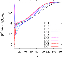
Figure 7. Flux differences  for all of the TH experiments. Ordinate is normalized by the potential enstrophy dissipation rate ην.
Download figure:
Standard image High-resolution image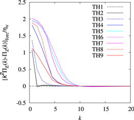
Figure 8. Contribution of the forcing spectra on the flux differences k2ΠE(k) − ΠZ(k) for all of the TH experiments. Ordinate is normalized by the potential enstrophy dissipation rate ην.
Download figure:
Standard image High-resolution imageWe have shown that the slopes of the simulated total energy spectra in the range k > kd are very close to those of the enstrophy inertial range and show no evidence of a transition to those of the energy inertial range. Furthermore, the Danilov inequality held for the whole wavenumber range. However, it is natural to ask whether or not either of these results could have been affected by the simulation resolution. To verify that these results were independent of the simulation resolution, we doubled the resolution and found no significant changes.
4.3. Effect of asymmetric hyper-viscosity
As described in section 3, asymmetric hyper-viscosity may lead to the Danilov inequality being violated. To investigate this issue, we performed six additional numerical simulations under the same conditions as for experiment TH2 but with different values of Δν. We shall refer to these experiments as the HV experiments, and the values of Δν used are listed in table 3. Table 4 lists the total energy and total potential enstrophy dissipation rates, as well as the total energies obtained for the HV experiments.
Table 3. Value of Δν used in the HV experiments.
| Experiment | HV1 | HV2 | HV3 | HV4 | HV5 | HV6 |
|---|---|---|---|---|---|---|
| (Δν)/ν | −0.9 | −0.75 | −0.5 | 1 | 3 | 9 |
Table 4. As for table 2, but for the HV experiments.
| Experiment | εκ | εν | ηκ | ην | E |
|---|---|---|---|---|---|
| HV1 | 0.908 103 · 10−1 | 0.199 789 · 10−2 | 0.120 674 · 101 | 0.425 145 · 102 | 0.284 280 · 101 |
| HV2 | 0.537 980 · 10−1 | 0.566 254 · 10−3 | 0.689 616 | 0.105 413 · 102 | 0.175 513 · 101 |
| HV3 | 0.881 833 · 10−1 | 0.458 950 · 10−3 | 0.984 288 | 0.777 483 · 101 | 0.265 538 · 101 |
| HV4 | 0.611 939 · 10−1 | 0.295 185 · 10−3 | 0.731 648 | 0.434 359 · 101 | 0.194 049 · 101 |
| HV5 | 0.575 895 · 10−1 | 0.242 090 · 10−3 | 0.694 527 | 0.348 647 · 101 | 0.182 183 · 101 |
| HV6 | 0.559 043 · 10−1 | 0.208 823 · 10−3 | 0.637 154 | 0.302 105 · 101 | 0.177 543 · 101 |
Similar to the TH experiments, both the energy and enstrophy dissipation wavenumbers are lower than the truncation wavenumber. In addition, the enstrophy dissipation wavenumber is higher than the energy dissipation wavenumber, and the transition wavenumber lies in the dissipation range, as found by the TH experiments. This therefore implies that the energy inertial range suggested by TO03 did not appear for kd ≲ k < kT in these experiments.
Figure 9 shows the dissipation spectra for all of the HV experiments, together with the spectrum for experiment TH2 for comparison. This shows that the dissipation spectra for TH2, HV4, HV5 and HV6 take their maximum values around the dissipation wavenumber kε and then decay sufficiently rapidly as the wavenumber increases further. In contrast, although the dissipation spectrum for HV3 also has a local extreme around kε, it starts to increase rapidly near the truncation wavenumber and takes its global maximum value there. Furthermore, the dissipation spectra for HV1 and HV2 do not even have local maxima around kε. We can therefore conclude that two of the experiments at least (HV1 and HV2) could not resolve the dissipation range.

Figure 9. As for figure 2, but for TH2 and all the HV experiments.
Download figure:
Standard image High-resolution imageFigure 10 shows the total energy spectra for all of the HV experiments, together with experiment TH2 for comparison. In all cases, these spectra follow power laws of the form  with δ ≃ 3 in the wavenumber range kd ≲ k ≲ kε. The spectra for HV4, HV5 and HV6 then decay smoothly as the wavenumber increases further, almost converging on the TH2 spectrum. In contrast, the slopes of the spectra for HV1, HV2 and HV3 become shallower for k ≳ kε as Δν decreases. In the cases of HV1 and HV2, we attribute this behavior to insufficient resolution in the dissipation range. As with the TH experiments, there is no evidence of the transition from E(k) ∼ k−δ to E(k) ∼ k−5/3 seen by TO03.
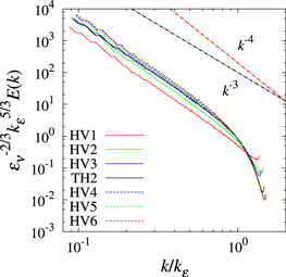
Figure 10. As for figure 5, but for TH2 and all the HV experiments.
Download figure:
Standard image High-resolution imageFinally, we consider the sign of the flux difference (1), as shown in figure 11. Again, the sign is negative in the entire range 1 ≤ k ≤ kT, i.e. the Danilov inequality held over the entire wavenumber range, even for the HV experiments.

Figure 11. As for figure 7, but for TH2 and all the HV experiments.
Download figure:
Standard image High-resolution image5. Conclusions and discussion
In this paper, we have used numerical simulations to investigate geostrophic turbulence governed by the two-layer QG potential vorticity equations forced by a horizontally homogeneous, baroclinically unstable basic flow. In particular, we have focused on the formation of the energy inertial range in the wavenumber range beyond kd and whether or not the Danilov inequality is violated. Despite conducting numerical simulations for wide throughput and asymmetric hyper-viscosity coefficient ranges, paying careful attention to both the budgets of the energy and enstrophy and the resolution of the dissipation range, we found no evidence of the energy inertial range or the violation of the Danilov inequality within reasonable numerical accuracy. Indeed, we found energy spectra that were close to the enstrophy inertial range spectra in the range kd ≲ k ≲ kε for large throughputs and approached k−4 as the throughput decreased. These energy spectra then decayed rapidly as the wavenumber increased further beyond the dissipation wavenumber kε.
The k−4 power-law shape of the total energy spectrum is reminiscent of the so-called Saffman spectrum (Saffman 1971). Saffman (1971) derived a k−4 energy spectrum for 2D NS turbulence with a discontinuous vorticity field. In fact, our numerical simulations indicate that the baroclinic component of the potential vorticity field in TH9 was nearly uniform with a steep transition region, as shown in figure 3(h). Furthermore, figure 4 shows that the baroclinic component dominated as the throughput decreased. This suggests that the k−4 total energy spectrum that we found for small throughputs can be interpreted as the Saffman spectrum. Venaille et al (2014) recently studied two-layer geostrophic turbulence in the limit of low throughput. They effectively described the formation of uniform potential vorticity with a steep transition region by both cascade phenomenology and statistical mechanical theory of the QG model.
Although the present study was motivated by TO03, the numerical simulations in the present study did not follow their simulations. TO03 conducted their simulations with channel geometry and adopted parameter values that mimicked realistic atmospheric conditions. In contrast, our goal was to investigate the validity of the Danilov inequality, independent of both flow domain geometry and boundary conditions. We thus adopted a square flow domain with cyclic boundary conditions. Furthermore, we conducted numerical simulations over wide throughput and hyper-viscosity coefficient ranges to study whether or not the Danilov inequality was a universal characteristic of two-layer geostrophic turbulence. It would be difficult to show that the present results are independent of both flow domain geometry and boundary conditions without conducting additional simulations, but simulations conducted by Thompson and Young (2006) imply that this should indeed be the case. They simulated the same two-layer QG potential vorticity equations as in our model, focusing especially on one of the fundamental turbulence properties, potential vorticity flux. They found that the potential vorticity flux was independent of the flow domain size for small throughputs, but began to depend on it for larger throughputs, calling these the local and global mixing regimes, respectively. The critical throughput value that divided these two regimes was nearly 12.5. All our numerical experiments, except for the TH1 experiment, were performed for throughputs below this critical throughput value. This suggests that our conclusions (except for those related to experiment TH1) are independent of both flow domain geometry and boundary conditions. In contrast, the estimated throughputs used in the TO03 experiments were nearly 27.3, as stated in section 4.1. So their results would have been influenced by both flow domain geometry and boundary conditions, potentially explaining both the Danilov inequality violation and the k−5/3 spectrum that they found. To confirm these conjectures, additional numerical simulations with channel geometry will be required and this will be the subject of our future studies.
TO03 introduced the flux difference as a measure for the extent to which the total energy flux dominates the total potential enstrophy flux. However, physical interpretations of the flux difference and the Danilov inequality have not been fully understood yet. Using the relation between the energy and enstrophy spectra, the Danilov inequality (3) can be rewritten as

for the 2D NS system. The relation (54) holds not only for the 2D NS system, but for generalized 2D fluids, the so-called α-turbulence system (Pierrehumbert et al 1994, Gkioulekas and Tung 2007). For the generalized 2D fluids, E(k) and Z(k) should be interpreted as the generalized energy and generalized enstrophy spectra, respectively, and  and ΠZ(k) are their fluxes. The relation (54) would be regarded as a generalized form of the Danilov inequality. Moreover, it would indicate that an effective flux of the energy in wavenumber space is less than those of the enstrophy. From the above discussion on a generalization of the flux difference, it is natural to ask whether (54) holds for the two-layer QG system, although the relation
  does not hold for the QG system. Here, E(k) and Z(k) should be interpreted as the total energy and total potential enstrophy spectra, respectively, and ΠE(k) and ΠZ(k) are their fluxes. In fact, as shown in figure 12, the results of the present numerical simulations also support (54) across the whole wavenumber range for all of the TH experiments. That is, the present numerical simulations suggest a generalized form of the Danilov inequality (54), which is applicable to 2D NS, α and two-layer QG turbulences.

Figure 12. Generalized form of the flux difference for the TH experiments.
Download figure:
Standard image High-resolution image
This paper has shown that the Danilov inequality is potentially valuable in describing energy and enstrophy cascades and avoids the restrictions of traditional arguments such as that of Fjørtoft's argument, which relies on triad interactions. However, it may not be possible to prove without very restrictive assumptions a Danilov inequality for systems more complicated than 2D NS. Even in the absence of a proof of the Danilov inequality, it would be useful to consider in numerical simulations the quantities represented in the Danilov inequality.
Acknowledgments
The main part of the present study was conducted when T I belonged to Kobe University. T I would like to thank all of the members of the Atmospheric Science Group of Kobe University for helpful conversations on this topic. We would like to thank two anonymous reviewers for their constructive suggestions. This study was partly supported by a Grant-in-Aid for Scientific Research (C) No. 15K05288 from the Japan Society for the Promotion of Science. T I was supported by funds No. 195002 from the Central Research Institute of Fukuoka University.
Appendix A.: Derivation of (16)–(25)
Substituting (14) and (15) into (10)–(13) yields the Fourier space versions of the governing equations, as follows:
Here,  , and
, and  , and the asterisks denote the complex conjugates. For brevity, the time argument has been omitted.
By multiplying (A.1) by  and adding the resulting equation to its complex conjugate, we obtain the following evolution equation for the modal barotropic energy:


Here, ![${\mathfrak{Re}}[A]$](https://content.cld.iop.org/journals/1873-7005/51/5/055507/revision2/fdrab2eadieqn60.gif) and
and ![${\mathfrak{Im}}[A]$](https://content.cld.iop.org/journals/1873-7005/51/5/055507/revision2/fdrab2eadieqn61.gif) represent the real and imaginary parts of the complex quantity A, respectively. The triads comprising only the barotropic modes are referred to as the barotropic triads and those including the baroclinic modes are referred to as the baroclinic triads.
represent the real and imaginary parts of the complex quantity A, respectively. The triads comprising only the barotropic modes are referred to as the barotropic triads and those including the baroclinic modes are referred to as the baroclinic triads.
By multiplying (A.2) by  and adding the resulting equation to its complex conjugate, we similarly obtain the following evolution equation for the modal baroclinic energy:


By adding (A.3) and (A.8), we obtain the evolution equation for the modal total energy, (16)–(20). Since the third term on the right-hand side of (A.3) cancels the fourth term on the right-hand side of (A.8), these do not contribute to the modal total energy budget.
Multiplying (A.3) by k2 and (A.8) by  yields the evolution equations for the modal barotropic and baroclinic potential enstrophies, respectively. In addition, by adding these equations, we can obtain the evolution equation for the modal total potential enstrophy, (21)–(25).
Appendix B.: Estimate of the throughput used in Tung and Orlando (2003)
Here, we estimate the throughput used in TO03. They considered a fluid confined to a mid-latitude channel centered at a latitude of ϕ0 = 50° on the Earth, with a zonal length of Lx = 25,700 km and width of Ly = 3340 km. Those correspond to the length of the circle of latitude at ϕ0 and the length of the meridian between 35◦ and 65◦, respectively. They scaled the spatial coordinates by Ly/π = 1.06 × 10⁶ m and the time by the inverse of the Coriolis parameter,  . In addition, their basic state assumed a cross-channel temperature difference of 57 K. We can derive the wind shear corresponding to this difference using the thermal wind relation, which in pressure coordinate is given by

where u is the zonal velocity, p is the pressure, T is the temperature and R is the gas constant per unit mass (e.g. Vallis 2006). Applying (B.1) to the 500 hPa level (between 250 and 750 hPa levels) leads to a zonal velocity difference of  between them. Furthermore, TO03 adopted an e-folding time for the Ekman friction of 6.7 d, with a static stability parameter σ0 of 0.193, which is a typical in winter values. Their parameters Δu, ν and σ0 correspond to our 2U, κ/2 and
  values, respectively. Scaling the spacial and temporal scales using the above values leads to U = 1.84 × 10⁻¹, κ = 3.08 × 10⁻² and kd = 2.28. Therefore, their throughput was (2Ukd)/κ = 27.2, which corresponds to the throughput of our experiment TH1.
Appendix C.: Detailed conservation laws for the energy and potential enstrophy
The following detailed energy conservation laws are satisfied by wavenumber triads that satisfy  :
:


In addition, the following detailed potential enstrophy conservation laws are satisfied by the same wavenumber triads:


Since it is computationally difficult to check the above detailed conservation laws for all possible triads, even with a state-of-the-art computer, we instead examine their sums over the whole wavenumber range:


Here,  indicates the summation of the quantity A over the whole wavenumber space. We have confirmed that the above conservation laws hold to within numerical accuracy.
Footnotes
- 4