Abstract
Dicke states are completely symmetric states of multiple qubits (2-level systems), and qudit Dicke states are their d-level generalization. We define here q-deformed qudit Dicke states using the quantum algebra  . We show that these states can be compactly expressed as a weighted sum over permutations with q-factors involving the so-called inversion number, an important permutation statistic in Combinatorics. We use this result to compute the bipartite entanglement entropy of these states. We also discuss the preparation of these states on a quantum computer, and show that introducing a q-dependence does not change the circuit gate count.

Original content from this work may be used under the terms of the Creative Commons Attribution 4.0 license. Any further distribution of this work must maintain attribution to the author(s) and the title of the work, journal citation and DOI.
1. Introduction
Completely symmetric multi-qubit states are called Dicke states. These highly entangled states have long been exploited for a wide variety of tasks in quantum information and computation, including quantum networking, quantum metrology, quantum compression, quantum tomography, and quantum optimization see e.g. [1–9], with specific interest in their entanglement characterizations [10–12], as well as methods of constructing these states in the lab [4, 13, 14] and on a quantum computer [15–18]. There has been growing interest in using d-level systems called qudits for quantum computation, see e.g. [19–24] and references therein. Completely symmetric multi-qudit states, which we call qudit Dicke states (also known as generalized Dicke states, or symmetric basis states), have also been studied for many years, see e.g [25–32].
In order to specify such multi-qudit Dicke states, it is convenient to introduce some notation. Let  , where ki
are non-negative integers, and
 is the number of qudits. Let
 denote the multiset

where ki
is the multiplicity of i, and let  denote the set of permutations of
 , which has cardinality equal to the multinomial [33]

The qudit Dicke states can then be expressed as [25–32]

where we sum over all permutations w of  . For example, the qudit Dicke state with d = 3, n = 4 and
 is

where as usual the tensor product is understood, e.g.  , and the computational basis states are denoted by
 , see (3.1).
We consider in this paper a q-analog of qudit Dicke states, which we call q-qudit Dicke states. In principle, there are many possible one-parameter (q) deformations of qudit Dicke states, which reduce to (1.3) in the limit q → 1. We consider here a particular deformation based on Quantum Groups, which has a number of attractive features, as we will see. The qubit case (d = 2) has been considered in [34]. Our main result is a formula (3.12) that generalizes (1.3) for q-qudit Dicke states, namely

where  denotes the inversion number and
 the maximum inversion number, see sections 2 and 3 for more details. We use this result to compute the entanglement entropy of q-qudit Dicke states (4.7). The inversion number is an important permutation statistic in Combinatorics [33]; it is interesting to see that it and the related q-combinatorial identities (3.17) and (4.6) appear in Quantum Information. We expect that q-qudit Dicke states will find applications similar to those of their undeformed (q = 1) counterparts, but with the advantage of having available a free parameter q as an additional degree of freedom.
This paper is organized as follows. In section 2 we briefly review  , the q-deformation of the su(d) algebra. In section 3 we use the generators of
 to define q-qudit Dicke states, and we note their key properties. In particular, we note a recursion relation for q-qudit Dicke states (3.8) (proved in appendix
2. Review of 

We briefly review here the  algebra with q > 0, following [35, 36], which we will use in the following section to define q-qudit Dicke states.
For a single qudit, the generators of the quantum algebra  are the same as for the classical (undeformed) algebra. In particular, we define the Cartan generators

and the Chevalley generators

where eij
are elementary d × d matrices with matrix elements  . Other generators can be obtained by taking commutators.
For n qudits, living in the vector space  , the corresponding generators are given by the coproducts [35, 36]


 , where
 is the d × d identity matrix,
 and
 occur at the jth location, and we sum j over all n positions. It is important to note for the next section that
 may be defined recursively

The algebra includes the commutator relations


where we use the bracket notation

so that  is symmetric under
 . It is clear that
 as q → 1, so that
 is a q-deformation of x. For more details about
 , see e.g. [35, 36].
3. q-qudit Dicke states
We define here q-qudit Dicke states, and note some of their key properties, including the recursion formula (3.8), the sum formula (3.12) and its extension to complex values of q (3.19), and the duality symmetry (3.22).
The single-qudit computational basis states are given as usual by the d-dimensional vectors

The single-qudit operators defined in (2.1), (2.2) perform the following mappings on these basis states:


3.1. Definition and recursive property
We use the  generators (2.3) and (2.4) to define the q-qudit Dicke states for fixed q > 0 and
 by the ‘operator formula’
1

where  denotes the q-multinomial

and the q-factorial is defined for non-negative integers n by

Indeed, for a single qudit, it is easy to see that the nested commutator  lowers the basis state
 to
 , i.e.
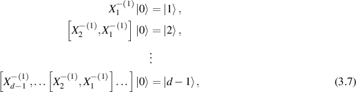
where the basis states are defined in (3.1). Hence, for  , the formula (3.4) can be seen to give the qudit Dicke state (1.3).
2
The q-qudit Dicke state (3.4) satisfies the important recursion

with the initial conditions  as given in (3.7), where
 is the sth unit vector in d dimensions

In the sum over s in (3.8), we implicitly skip over s = i if  , since
 is then not defined. A detailed proof of this recursion is given in appendix
 in (2.5). As we shall see in section 5, it is due to the recursive nature of the q-qudit Dicke states that these states can be efficiently generated on a quantum computer.
3.2. Sum formula
The q-qudit Dicke states can be written explicitly in terms of permutations, generalizing the q = 1 result (1.3). To do so, we need to borrow a notion from Combinatorics (see, e.g. [33]). Every permutation w of  can be regarded as a ‘word’ with n ‘letters’ wi
in the alphabet
 , i.e.
 . We refer to the permutation in weakly increasing order, satisfying
 for all i < j, e.g. 0112, as the identity permutation
 . The inversion number of a permutation w, written
 , represents the minimum number of adjacent transpositions it takes to go from the identity permutation to w. The inversion number of w can be efficiently computed by

where zj
equals the number of letters  satisfying i < j; that is zj
is the number of letters to the left of wj
larger than wj
. For example, for w = 1201, we have
 ; thus
 ; and hence
 .
We let  denote the maximum inversion number of all permutations of
 ; clearly this corresponds to the permutation in reverse-order of the identity permutation
 (i.e. weakly decreasing). Thus

where the term  with i < j represents the
 ’s to the left of the
 ’s in the reverse of the identity.
We claim that the q-qudit Dicke states (3.4) may be expressed by the ‘sum formula’

where we sum over all permutations w of  . For example, the q-qudit Dicke state corresponding to (1.4) with
 is

To prove that the sum formula (3.12) is valid, all we need to do is show that this formula satisfies the recursion in (3.8) along with the same initial conditions. Clearly, (3.12) has the same initial conditions  . Note that any permutation w that ends with the letter s can be expressed as
 , where ws
is a permutation of
 . The inversion numbers for w and ws
are related by

where the sum denotes the number of adjacent transpositions it takes to move the right-most s in the identity permutation  to the nth position, obtaining
 . Let
 denote the corresponding maximum inversion number over all ws
. Then
 because

The sum  represents the number of non-s letters that cross over the right-most s in
 when reversing the identity permutation
 . Substituting
 ,
 , and
 in terms of
 ,
 , and
 in (3.12), using the fact
 , and summing over all possible s, we see that (3.12) satisfies recursion (3.8). That the factor with
 is present in front of
 in (3.12) is not entirely surprising, as the proof of the recursion of the q-qudit Dicke states (see appendix
The sum formula (3.12) makes clear the orthogonality of any pair of q-qudit Dicke states with different  ’s. The identity
3

confirms that the q-qudit Dicke states (3.12) are normalized to unity, and thus are orthonormal. This identity also shows that the q-multinomial can be expressed as a Laurent polynomial in q with non-negative integer coefficients cf the denominator in (3.13), which is a nontrivial generalization of the fact  for positive integers n.
3.3. Complex q
We have so far assumed that the deformation parameter q is positive q > 0. Let us now briefly consider a complex deformation parameter  , with
 and α real. It is not obvious how to define corresponding q-qudit Dicke states; indeed, replacing q by q in (3.4) could lead to complications if q is a root of unity, i.e.
 for some positive integer p, since then
 . We therefore define q-qudit Dicke states instead by the recursion (3.8) with q replaced by q, i.e.

where the brackets are given by (2.8) with  , which is well-defined (after choosing the square-root branch cut) even if q is a root of unity. It follows that

where again the brackets are given by (2.8) with  .
As an example, let us consider the case  with
 . The brackets are to be computed with the absolute value of q; that is, with
 . Therefore,

and the q-qudit Dicke state (3.19) is given by

Note that defining the q-qudit Dicke states by (3.18) ensures that they are properly normalized  , where as usual
 and
 is given by the complex conjugate of q. The special case
 , which corresponds to antisymmetric states, has been considered in the literature, see e.g. [25, 27, 31, 37] and references therein.
3.4. Duality symmetry
The sum formula (3.19) can be used to show that the q-qudit Dicke states have the ‘duality’ symmetry

where

denotes the reverse of  , and
 is the d × d antidiagonal ‘charge conjugation’ matrix

which performs the mapping

on the single-qudit basis states (3.1). This is a generalization of the well-known duality property of qubit Dicke states  .
4. Entanglement entropy
Quantum entanglement is a key resource of Quantum Information. An important measure of quantum entanglement is the bipartite entanglement entropy, see e.g. the reviews [38, 39]. For qubit Dicke states ( ), the bipartite entanglement entropy was computed in [10–12]; this result was generalized for qudit Dicke states (general d, but q = 1) in [26, 30]. Moreover, the generalization to q-qubit Dicke states (
 ) was done in [34]. We extend the entanglement entropy computation here to the general case of q-qudit Dicke states, with q > 0; in fact, for the case of complex q where the states are given by (3.19), the entropy has a similar form as the case
 .
In order to compute the Von Neumann bipartite entanglement entropy, we begin by finding the Schmidt decomposition of the q-qudit Dicke states. We recall that the d-tuple  consists of non-negative integers ki
satisfying
 ;
 is then referred to as a weak d-composition of n [33], so that we can associate all weak compositions with q-qudit Dicke states. For example,
 is a weak 3-composition of 4. We wish to partition the state with n qudits into two parts, with l and n − l qudits, for a positive integer l < n. Thus, given
 and l, we consider d-tuples
 that are weak d-compositions of l satisfying
 . We let
 denote the set of all such
 ; explicitly,

For example, for  and l = 2, we have
 . If
 then
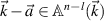 , i.e.
 is a weak d-composition of n − l satisfying
 ; it is now clear that the cardinality of
 is symmetric under
 . With these conditions, we have essentially ‘cut’
 into
 and
 . We can then associate the q-qudit Dicke states
 and
 with
 and
 .
The Schmidt decomposition of the q-qudit Dicke states for fixed l can be written as

with

A proof of this decomposition is given in appendix  can be understood as Clebsch-Gordon coefficients relating symmetric representations of
 . In the limit as
 reduces to the multivariate hypergeometric distribution [30], which has a clear combinatorial meaning: it represents the ratio of the number of permutations w of
 that contain in the first l positions the letters i with multiplicity ai
and in the last n − l positions the letters i with multiplicity
 to the number of all permutations w.
Let  be the density matrix of a pure q-qudit Dicke state, which in light of the Schmidt decomposition (4.2) can be expressed as

The reduced density matrix  is obtained by tracing over the last n − l qudits, which, using the orthonormality of the q-qudit Dicke states, forces
 . So

implying  is diagonal in the q-qudit Dicke state basis, with eigenvalues
 . The eigenvalues of a density matrix are non-negative and sum to unity, implying

which we recognize as the q-Vandermonde identity for multinomials 4 . The Von Neumann bipartite entanglement entropy is given by

where  is given by (4.3). For the general case of complex q, where the states are given by (3.19), the eigenvalues of
 are given by
 , which simplifies to
 with
 , see (4.3). It follows that the entanglement entropy for complex q is given by (4.7) with
 .
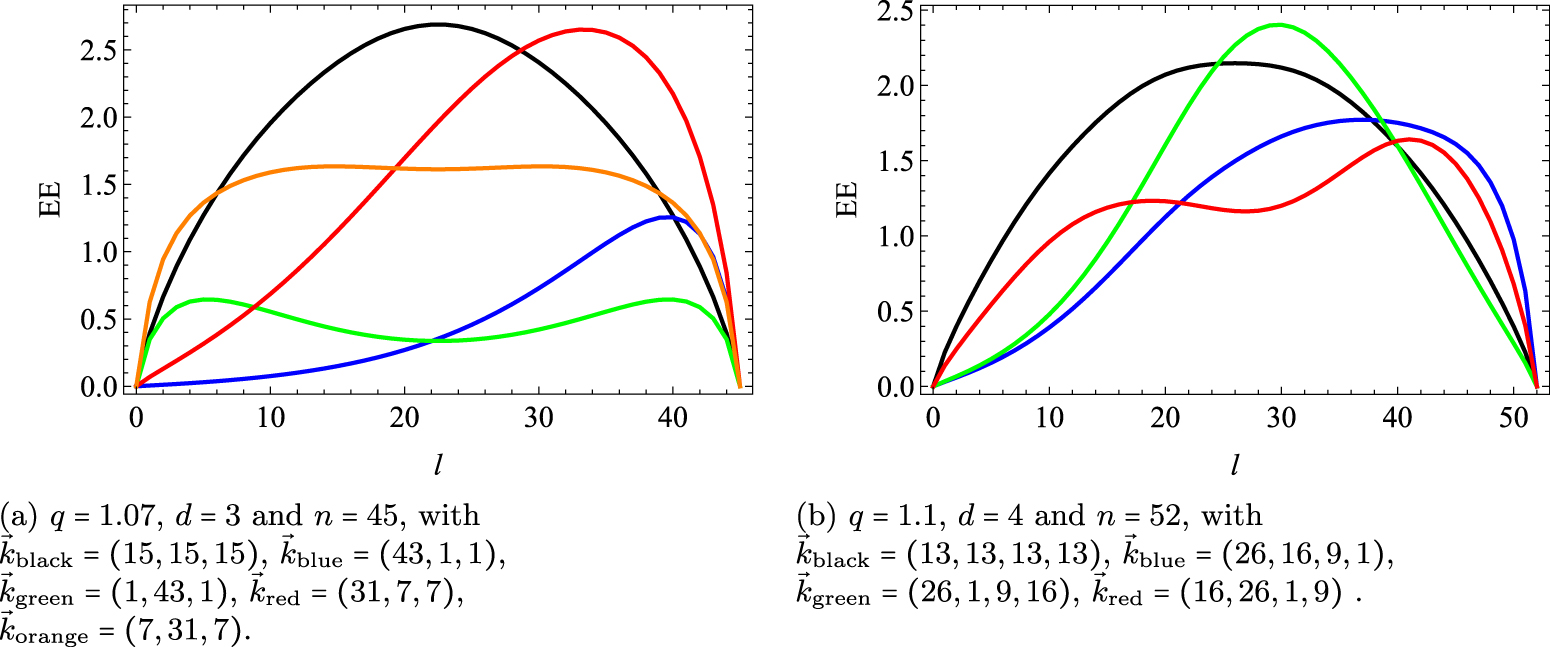
We compute the entanglement entropy (EE) (4.7) numerically, see e.g. figure 1. The symmetry  , which follows from the
 symmetry of the q-multinomial, induces the symmetry
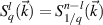 [34]. We thus restrict our attention to
 , as
 simply reflects the plot over
 . Further, we note the symmetry
 , corresponding to the duality symmetry (3.22). This implies that
 . The latter symmetry is exemplified by the black, green and orange curves in figure 1(a), whose
 ’s satisfy
 , and are therefore symmetric about
 .
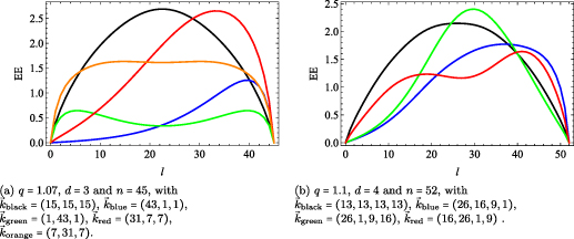
Figure 1. Entanglement entropy (EE) (4.7) of q-qudit Dicke states as a function of l.
Download figure:
Standard image High-resolution imageWe also see from figure 1(a) (blue vs red) that states whose  ’s have similar proportions (in this example,
 ) have EE curves (EE vs. l) with similar shape. On the contrary, we see from figure 1(b) that states whose
 ’s have different proportions (such as blue
 and red
 , which are related by a permutation) have EE curves with different shapes. Clearly, for a given value of n, larger values of d allow for more ways of choosing
 with different proportions. By suitably choosing d,
 and q, EE curves with a great variety of shapes can be obtained.
5. State preparation
The problem of preparing a general quantum state on a quantum computer [41, 42] (i.e. by acting with unitary transformations on a simple reference state) is interesting but difficult. For the case of qubit Dicke states ( ), an efficient deterministic algorithm has been developed, see [15–18] and references therein. A generalization to the case of qudits (general d , q = 1) was recently given in [32]. We consider here briefly the problem of preparing q-qudit Dicke states, and find that adding a q-dependence adds little difficulty to the algorithm. We begin by laying out the general approach for arbitrary d, and then work out in detail a suitable circuit for the case of qubits (d = 2). Finally, we show that this circuit can be simplified by removing certain gates.
5.1. General d
Similarly to [15, 32], we begin by looking for a unitary operator Un
(independent of  ) that generates
 for all
 by acting on the identity permutation
 ,

for all  , where
 with
 and
 real. The recursive nature of the q-qudit Dicke states (3.18)

indicates that Un
can be constructed recursively, as the q-qudit Dicke states on the LHS and RHS of (5.2) can be constructed by applying Un
and  to the states
 and
 (for all s), respectively. This motivates finding an operator Wn
(independent of
 ) that performs the mapping

for all  . In terms of this operator Wn
, we can clearly see the recursion

Using the initial condition  , we can telescope the recursion (5.4) into a product of Wm
operators

where the product goes from left to right with increasing m. The problem therefore reduces to constructing quantum circuits for the Wm operators.
5.2. d = 2
As an example, we consider the simplest case, namely d = 2 (qubits). We associate  with
 , so that (5.3) reduces to finding a gate decomposition for Wm
(
 ) that satisfies
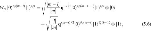
for all  (Wm
acts as the identity when l = 0 or l = m), where as before the brackets are given by (2.8) with
 . We introduce the operator
 acting on the lth,
 th, and 0th qubit, that performs the transformation
5

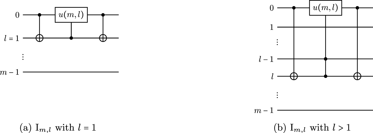
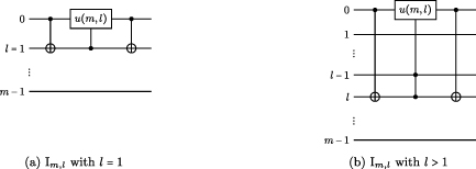
and otherwise acts as identity (as long as the 0th qubit is in the state  ). The corresponding circuit diagram is given by figure 2, with one-qubit unitary u-gates

whose angles  depend on
 as follows:

In this section, following Qiskit conventions, we label m-qubit vector spaces from 0 to m − 1, going from right to left; and in circuit diagrams, the m vector spaces are represented by corresponding wires labeled from the top (0) to the bottom  .


Download figure:
Standard image High-resolution imageNote that the identity permutation  remains invariant under
 , i.e.
 , if
 ; further
 remains invariant as well,

Hence, a quantum circuit that performs the transformation (5.6) for all  is given by an ordered product of such operators

where the product goes from right to left with increasing l.
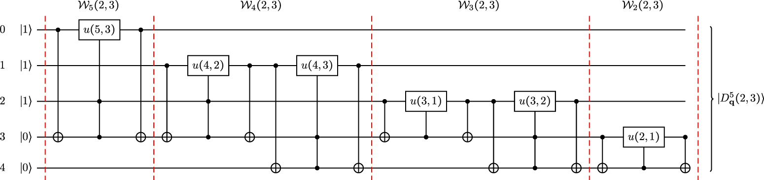
As an explicit example with n = 5, we see from (5.5) that

and the corresponding complete circuit diagram is shown in figure 3. This circuit can be used to prepare the 5-qubit q-Dicke state  from the initial state
 for any
 . For the particular case l = 3, the shaded gates are redundant and can therefore be removed, as explained below.

Figure 3. Circuit diagram for U5 (5.12), with W’s (separated by red dashed lines) given by (5.11) in terms of  ’s in figure 2. This circuit can be used to prepare the state
 for any
 . For the particulr case l = 3, the shaded gates can be removed.
Download figure:
Standard image High-resolution image5.2.1. Simplifying the operators.
While the Un
operator (5.5) in terms of Wm
’s (5.11) does generate a q-qubit Dicke state for any  , its gate count can generally be reduced. Indeed, we now proceed to prune away the redundant gates, and thereby remain with a simplified operator
 in terms of corresponding simplified operators
 , such that

which are tailored for a fixed value of l. We begin by considering how the right-most factor in (5.5), Wn
, acts on  for a fixed l. It is clear that we can remove n − 2 factors in the product (5.11), simplifying to
 . For example, for l = 3 in figure 3, we can remove gates
 in W5.
We next consider how  acts on
 . Rewriting (5.11) as

we find that all the terms in the right-most product can be removed, as their controls are in qubit positions between and including 1 and l − 1, where the qubits take the value of  . For example, for l = 3 in figure 3, the term
 in W4 can be removed, as the controls lie on wires 1 and 2. Similarly, the terms in the left-most product can be removed as they also never get activated. Thus, the factor
 in (5.5) can be simplified to
 .
Similar analysis can be done on the general Wm factors in the product (5.5), leading us to generalize [15] to q-qubit Dicke states by creating the quantum circuit for fixed l

where

performs the transformation (5.6) for a fixed l. Note that the presence of max/min in (5.16) is simply enforcing the requirement  in
 .
The number of  -gates in
 is given by

which satisfies  , and
 for
 . We see that there is no gate count advantage to using the dual symmetry (3.22)
 as the gate count is symmetric under
 . However, by using the dual symmetry to restrict to
 , one can minimize the separation of the wires on which the
 -gates act.
Considering as an example the particular case  , we see from equations (5.13) and (5.15) that
 , with

where the  ’s are given by (5.16), as shown in figure 4. Note that this circuit can be obtained by removing the shaded gates from the circuit in figure 3. An implementation in Qiskit of this and additional examples, as well as Mathematica code for verifying the results, are available as supplementary material.
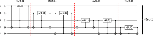
Figure 4. Circuit diagram for preparing the state  , where
 is given by (5.18) and the
 ’s (separated by red dashed lines) are given by (5.16) in terms of
 ’s in figure 2.
Download figure:
Standard image High-resolution imageNote that the only dependence on q is through the angles in the  gates (5.8); hence, the gate count for general q is the same as for
 [15–18]. For d > 2, we expect that the q-dependence can be implemented in a similar way.
6. Conclusion
We have used Quantum Groups to define the notion of q-qudit Dicke states through the operator formula (3.4), and we have shown that these states can be expressed by the compact and useful sum formula (3.12). A key ingredient of the latter is the inversion number, which is an important permutation statistic in Combinatorics. Basic properties of these states and their bipartitions are expressed by celebrated q-combinatorial identities (3.17), (4.6). This interplay among Quantum Groups, Combinatorics and Quantum Information suggests that there may be deeper relations among these subjects.
We have seen that the recursive nature of the q-qudit Dicke states (3.8) leads to a simple algorithm for their construction on a quantum computer. We note that the Schmidt decomposition (4.2) can be regarded as a generalization of this recursion; indeed, (3.8) can be obtained by letting  in (4.2). It should be possible to further generalize the Schmidt decomposition of q-qudit Dicke states to multipartite decompositions, and study multipartite entanglement. It would be interesting to see if other algorithms can be obtained by similarly exploiting these generalizations of the recursion (3.8). It may also be possible to compute the
 limit of the bipartite entanglement entropy with q > 0, as has been done for the undeformed (q = 1) case in [10, 11, 26, 30].
As noted in the introduction, Dicke states have been exploited for numerous tasks in quantum information and computation. We expect that q-qudit Dicke states will find similar applications, but with the advantage of having available a free parameter q as an additional degree of freedom. Larger values of d will allow for more choices of  , and therefore richer structure, see e.g. figure 1. As discussed in section 5, the preparation of such states is not much more difficult than for undeformed qudit Dicke states.
Acknowledgments
We thank Galib Hoq for his collaboration at an early stage of this project, and Michelle Wachs for valuable correspondence. R N was supported in part by the National Science Foundation under Grant No. PHY 2310594 and by a Cooper fellowship.
Data availability statement
All data that support the findings of this study are included within the article (and any supplementary files).
Appendix A: Proof of the recursion (3.8)
We show here that the q-qudit Dicke state (3.4) satisfies the recursion (3.8). We begin by introducing in section A.1 new operators, in terms of which the expression for the q-qudit Dicke state takes the simpler form (A.12). We then evaluate this expression in section A.2 to arrive at the desired result (3.8).
A.1. New operators and their properties
Let us recall that the single-qudit operators  (2.1) and
 (2.2) perform the mappings (3.2) and (3.3), respectively, on the computational basis states. We now define new operators on n qudits
6


which, for n = 1, perform the mappings


It is natural to wonder if the  operators satisfy relations analogous to (2.4) and (2.5). In fact,


where ‘rem’ denotes additional remainder terms that vanish when applied to the state  , where
 denotes an arbitrary sum of kets of n qudits with each ket consisting of 0’s, i’s, j’s, etc. This may be understood by substituting (2.4) into (A.1):

When the products are expanded into a sum of terms, each such term will have exactly i operators  ’s spread throughout the n locations. The n terms for which the
 ’s occur at the same location together form the square-brackets term in (A.5). The rest of the terms have an interrupted sequence of lowering operators at some location (e.g. the expansion of
 includes terms which at some location equals
 , which is missing
 ) and thus acts trivially on the state
 using (3.3).
We conclude this subsection with two useful claims.

where ‘rem’ denotes additional terms that vanish when applied to the state
 .
7
To show this, we compute the commutator

where we used (A.5) (valid when acting on  ) and that
 commutes with
 . Now, using (A.4)

acting trivially on states other than  due to (A.3). So the factor
 to the right of the commutator at location k in (A.9) necessarily produces the factor
 ; thus

Using  , our claim (A.8) follows.


We can illustrate this result by expanding all of the commutators of  in the last factor of (3.4). One of the expanded terms is the ordered product
 , which acting on
 becomes
 . The rest of the terms contain an out-of-order product, e.g.
 . Each of these terms acts trivially on the state
 in light of (3.3). It is thus easily seen that the last factor in (3.4) may be written as

The second-to-last factor in (3.4) acts similarly on the state  , with the only non-trivial term being
 , producing the state
 . Continuing in this fashion justifies (A.12).

A.2. Evaluation of (A.12)
We now proceed to (partially) evaluate (A.12), which will lead to the recursion (3.8), repeated here for convenience

Using (A.6), (A.3) and (A.4), we see that

where we have applied to  a single power of
 . Applying a second power gives us the terms

We now use (A.8) to compute the interchange of 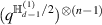 and
 ; this single interchange produces the factor q−1, and thus our terms (A.16) simplify to

It is clear that if we apply another power of  , we will generate the term
 , which requires two interchanges, generating a factor of q−2. After applying l powers of
 , we have

where the coefficient cl satisfies

and therefore

Taking  in (A.18), we obtain

Noting from (A.6), (A.3) and (A.4) that

we see from (A.12) and (A.21) that
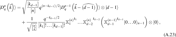
where the first term is the last term in the sum in the recursion (A.14).
We now compute the effect of  in (A.23). Applying one power of
 , we use again (A.6) to obtain
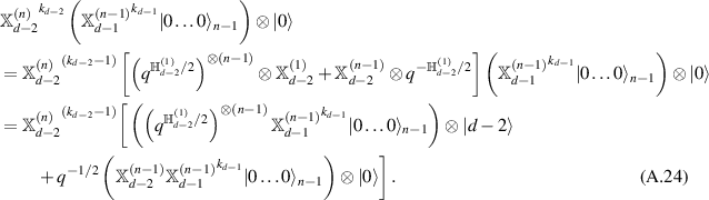
We now need to perform  interchanges of
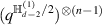 and
 , each of which produces a factor of
 , see (A.8). Applying a second power of
 will produce a term with the factor
 , where the q−1 comes from the additional interchange of
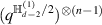 and
 , etc. Thus
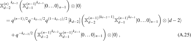
cf (A.21). Substituting this result into (A.23) produces the second term in the recursion (A.14). It is not difficult to continue this argument to generate the rest of the terms in the recursion. 
Appendix B: Proof of the Schmidt decomposition (4.2)
The proof of (4.2) follows from a generalization of an argument below equation (A.9) in [30] for q = 1. Recall that the q-qudit Dicke states can be expressed by the sum formula (3.12)

Every permutation w can be split into  , where
 and
 are respectively permutations of
 and
 , where
 (4.1). We can then split the sum over permutations w of
 into sums over all
 , over permutations wa
of
 , and permutations wb
of
 ; explicitly,

The inversion numbers of w, wa , and wb are related by

where the term 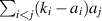 represents the minimum number of adjacent transpositions needed to go from
 to
 , where
 denotes the identity permutation corresponding to
 , and similarly for
 and
 . Indeed, starting from the identity permutation

we move  letters d − 2 from left to right (past the dashed vertical line) across
 letters d − 1, thereby arriving at

which entails  adjacent transpositions. We continue successively moving
 letters
 from left to right across all aj
letters j > i, until we arrive at

which entails a total number of adjacent transpositions given by 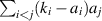 .
Substituting (B.2) and (B.3) into (B.1), we obtain
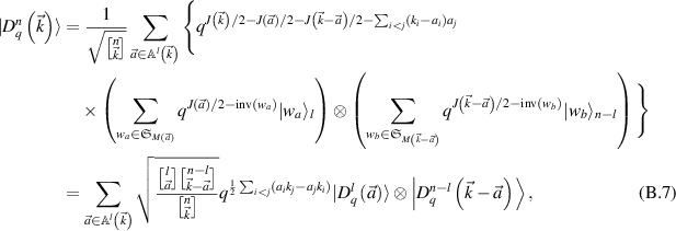
where we have passed to the last line using (3.11). 
Footnotes
- 1
We occasionally place a subscript n on a ket, such as
in (3.4), to clarify that it is a state of n qudits. - 2
A proof of this fact follows from the
limit of (3.12). - 3
This identity has a long and interesting history recounted in [33]. In equation (1.68) of [33], this identity is written in the form
where the boldface denotes the
-multinomial using a definition of -deformation that is different from (2.8), namely where the q in is evaluated at . Computing using and using gives . Substituting this into (3.16) and letting leads to our form (3.17). - 4
See e.g. proposition 2.6 of [40]. To convert between different q-deformations, see footnote 3.
- 5
For l = 1, the middle qubits in (5.7) are omitted.
- 6
We write
in place of for notational convenience. - 7
We conjecture that the additional terms are absent, i.e. that the result (A.8) is actually a strict equality. However, we do not need the stronger result here.