

Abstract
This study aims to develop a novel mathematical epidemic compartmental model that includes a compartment or class for individuals who become infected and experience severe illness due to the infection. These individuals require hospitalization and the use of specialized medical equipment, such as ventilators, ICU beds, etc, during an outbreak. This compartment is referred to as the 'hospitalized population compartment' throughout this study. Additionally, the model incorporates a saturated incidence rate for new infection cases and the hospitalization rate for individuals severely affected by the infection, intending to create a more realistic scenario of the dynamics of disease transmission. The model is developed by integrating a compartment for hospitalized individuals into the standard susceptible-infected-recovered compartmental model and is subsequently mathematically analyzed for qualitative behavior. In this model, the saturated hospitalization rate reflects that the number of severely infected individuals who can be hospitalized is limited at any given time due to constraints in sufficient hospital infrastructure availability. The incidence rate of susceptibles becoming infected is modeled using the Holling Type II functional form, which incorporates inhibitory effects observed within the population. The study analyzes the mathematical model for two types of equilibria: the disease-free equilibrium (DFE) and the endemic equilibrium (EE). To investigate the stability of both equilibria, the basic reproduction number,  , is calculated using the next-generation matrix method. The findings indicate that when
  , the DFE is locally asymptotically stable. Conversely, when
  , the DFE becomes unstable, leading to the emergence of a positive EE. Additionally, the study explores the occurrence of forward and backward transcritical bifurcations under specific conditions when
  . Furthermore, the study delves into both the local and global stability behaviors of the EE. Numerical simulations of the model are also performed to support the theoretical findings.
Export citation and abstract BibTeX RIS
1. Introduction
Whenever an epidemic outbreak occurs in society, it is of paramount importance for the government and healthcare workers to take swift action to control the spread of the disease and provide medical treatment to infected individuals. Mathematical modeling plays a vital role in understanding and predicting the spread of the disease, with numerous models such as SIS, SIR, SIRS, SEIR, SEIRS, SEIQ, SVIRS,  , and others that have been proposed in the epidemiology literature [1–15]. These models use different variables such as susceptible, vaccinated, infected, exposed, quarantined, infodemic, and recovered individuals to represent different stages of disease progression. The dynamics of these models are largely determined by the rates of incidence, contact, and recovery. Amongst these, the incidence rate, which represents the rate of new infections, is of critical importance. Generally, the incidence rate is proportionate to the number of susceptible and infectious people. In 1927, Kermack and McKendrick [16] proposed a SIR epidemic model with a bilinear incidence rate
  ; however, this model is ineffective in cases of overcrowded infectives. The bilinear incidence rate assumes that the contact rate and infection probability per contact remain constant over time, which does not reflect reality. The number of infective individuals greatly influences individual mobility as it represents the risk of infection. As an example, during the SARS outbreak in 2003, as the number of SARS-infected individuals increased, various protective measures and control policies such as closing schools, restaurants, and postponing conferences were implemented. These measures significantly reduced the number of contacts per unit of time, thus lowering the incidence rate [17]. Hence, it is essential to consider the infection force, which includes individuals' adaptation to infection risks, in the modeling of disease dynamics. Therefore, to address the limitations of traditional models and more accurately capture the complexities of disease transmission dynamics, Capasso and Serio [18] introduced a revolutionary concept in 1978: the saturated incidence rate
  into the disease transmission model. This innovative approach takes into account the real-world phenomenon of saturation, where the rate of infection tends to level off as the number of infected individuals increases. The saturated transmission infection force, represented by the equation
  , effectively accounts for the decrease in contact rate and infection probability per contact as the number of infective individuals increases. This provides a more accurate representation of the actual spread of the disease. The
  in
in  estimates the infection force, while
  measures the impact of behavioral changes in susceptible individuals due to increasing numbers or the density effect of infective individuals. The idea of incorporating the saturated incidence rate
  into the disease transmission model represents a significant advancement in the field of epidemiology. It is a more sensible approach than the traditional bilinear incidence rate
  [9] as it accounts for the crucial real-world phenomenon of behavioral change and the crowding effect of infective individuals. This approach also retains the unboundedness of the contact rate by choosing suitable parameters, providing a more accurate representation of the actual spread of the disease. Furthermore, the work by Capasso and Serio has been widely adopted by many researchers in the field, with numerous studies applying the saturated incidence rate to disease transmission dynamics in various epidemic models (see, for example [6, 19, 20]).
The recovery rate of infected individuals is a crucial factor in controlling the spread of disease and minimizing its impact on the population. This rate is primarily determined by the length of the recovery process, which is, in turn, related to the availability of good health infrastructure, such as the number of doctors, nurses, medicines, isolation areas, and available hospital beds per million populations. The availability of these resources is a key consideration for health planners in determining the level of treatment that can be provided to patients [21]. Unfortunately, limited health infrastructure or resources can have dire consequences, such as an increase in new infection cases, a rise in the death rate, and psychological effects on individuals' mental health. To characterize the saturation phenomenon of limited health infrastructure, a continually differentiable hospitalization rate function (Holling functional type II) is considered, represented by the equation  , where γ and δ are non-negative constants. The term
  measures the hospitalization rate of severely infected individuals, whereas the term
  gauges the limitation in the hospitalization of infected individuals due to the limited number of hospitals, isolation places, equipment, limitations of hospitals with required facilities, etc. The Holling type II functional form has been widely adopted in disease modeling. In 2008, Zhang and Liu [22] considered the treatment rate in saturated function form within their study. They proposed a SIR model using the following system of differential equations to describe the disease transmission dynamics:
In the above system of equations,  and
and  stand for the susceptible, infected, and recovered populations, respectively whereas the parameters
  and
and  represent the constant recruitment rate of the susceptible population, the natural mortality rate, the disease-induced mortality rate, the natural recovery rate of infected individuals, the transmission rate of infection, the psychological effects or inhibitory effects, the cure rate, and the extent of the effect of delayed treatment for the infected individuals, respectively. Moreover,
  , and
, and  represent the saturated incidence and treatment rates, respectively. Subsequently, in 2012, Zhou and Fan [23] modified the model of [22] by transforming the saturated treatment rate
  into the form
  to better represent the realistic aspect of capturing the effects of limited medical resources for infected individuals and they studied the qualitative behavior of the model with this revised term. Despite these advancements, previous studies have not addressed the significance of the hospitalized population class and its impact on disease transmission dynamics. It is more reasonable to incorporate a dedicated class into the model, as the inclusion of this class enables a more precise representation of disease propagation and progression. This approach can facilitate tracking the population under hospital care at any time, the mortality count during hospital treatment, and the population that recovers after receiving medical treatment in hospitals. Therefore, this study aims to bridge this gap by introducing a novel model that incorporates a distinct class for hospitalized individuals within the SIR (susceptible-infected-recovered) framework, utilizing a saturated hospitalization rate. Furthermore, this representation acknowledges the potential discrepancy in growth rates between individuals requiring hospitalization and those becoming infected. Aligning with the evolving understanding of disease transmission and the role of hospitals in disease management enhances the effectiveness of this approach.
The goal of this study is to introduce and mathematically analyze an epidemic model that considers the hospitalized population class for severely infected individuals, limitations in the hospitalization of the infected population, and inhibitory effects by the population for disease transmission dynamics. In the present study, the model is proposed by dividing the total population into four subpopulation compartments: susceptible, infected, hospitalized, and recovered individuals, based on their disease status. By incorporating a saturated incidence rate and a saturated hospitalization rate, the standard SIR model is extended into the  (susceptible-infected-hospitalized-recovered) model. We investigate the basic properties of the model solution. Moreover, the identification of equilibrium points and the computation of the basic reproduction number (BRN), denoted as
  [24, 25], are performed through Descartes's rule of signs and the Next-generation matrix method, respectively. The study examines the local and global stabilities of the equilibria using
  , the Routh–Hurwitz criterion, and the Lyapunov function method. Additionally, we perform a bifurcation analysis for the model's stability behavior. Furthermore, numerical results are provided to corroborate the theoretical findings.
The paper is structured as follows: section 2 presents the proposed mathematical model and its properties. Section 3 examines the local stability of the model equilibria, while section 4 specifically analyzes the global stability of the endemic equilibrium (EE) due to the study's revelation of a backward bifurcation at  . Section 5 supports the theoretical findings with numerical simulations, and section 6 explores the sensitivity of the BRN. Finally, section 7 concludes the paper with a summary of the findings and a discussion of their implications.
2. Mathematical framework and its properties
In this section, we present a nonlinear epidemic transmission model for disease transmission dynamics. To achieve this, the total population size  is divided into four distinct subpopulations: susceptible, infected, hospitalized, and recovered. Each subpopulation represents a different stage in the progression of the disease. The model considers the complex dynamics of disease transmission, assuming that the disease can only be transmitted to susceptibles through close contact. Furthermore, individuals who have recovered and gained immunity no longer contribute to the transmission process. The susceptible subpopulation comprises individuals susceptible to contracting the infection through close contact with infected individuals. Conversely, infected individuals possess the capacity to transmit the disease under specific circumstances. The hospitalized subpopulation encompasses individuals who suffer severe illness due to the infection, necessitating specialized care for recovery. Recovered individuals, conversely, have successfully fought off the infection and regained their health, either through auto-recovery or medical treatment. To illustrate the process of disease transmission among these subpopulations, a block diagram is presented in figure 1.

Figure 1. Transfer diagram of infection.
Download figure:
Standard image High-resolution imageThe transitions between subpopulations are mathematically expressed by the following system of ordinary differential equations, under the aforementioned assumptions:
with initial conditions:

In model (1), the rate of change in each subpopulation is represented by  , and the constant recruitment rate into the susceptible population is denoted by
  . The transmission rate of infection is represented by
  , while the rate of inhibition by the infected population is denoted by
  . The natural death rate in all subpopulations is symbolized by
  , and the hospitalization rate of severely ill infected individuals is indicated by
  . The rate of limitation in the hospitalization of critically ill patients due to inadequate health infrastructure is denoted by
  . The disease-induced death rate of infected individuals is denoted by
  , and the disease-induced death rate of infected individuals in hospitals during treatment is denoted by
  . The recovery rate of hospitalized individuals after medical treatment is represented by
  , and the auto-recovery rate of infected individuals is represented by
  . The term
  represents the saturated incidence rate at which susceptibles become infected when they come into close contact with infected individuals. In this term,
  represents the force of infection, and
  measures the inhibitory effects. If we consider no inhibitory effects (i.e.
  ), then
  simplifies to
  , which is a well-known bilinear incidence rate [16, 24]. The term
  represents the saturated hospitalization rate of severely infected individuals, where the parameters
  and
and  are both non-negative. Below table 1 is given for a comprehensive description of the variables and parameters of the model (1).
Table 1. Notation and corresponding explanations.
| Symbol | Description |
|---|---|

| Susceptible population. |

| Infected population. |

| Hospitalized population. |

| Recovered population. |

| Constant recruitment rate. |

| Natural death rate. |

| Transmission rate of infection. |

| Inhibition rate or effect. |

| Hospitalization rate of severely infected individuals. |

| Limitation rate for hospitalization of infected individuals. |

| Mortality rate due to disease among infected people. |

| Mortality rate due to disease among hospitalized people. |

| Auto-recovery rate of infected individuals. |

| Recovery rate of hospitalized individuals after medical treatment. |
The variables and parameters in model (1) are assumed to be non-negative and positive, respectively, in line with biological reasons. Furthermore, we have identified a region of attraction for the solutions of model (1) as described in lemma 1.
Lemma 1. The set  is a positive invariant set of the system (1) under condition (2).
Proof. By adding all equations of the model (1), we obtain
On integrating, we get
Therefore,  . Further,
  if
if  . It shows that solutions of the model (1) approach
  ,
,  is a positively invariant set and solutions of the model (1) are bounded, all provided
  .
.
Excluding the fourth equation from the aforementioned model (1) for mathematical analysis does not have a significant impact on the overall system dynamics, as variable  is absent in the first three equations of the model (1). Therefore, it is sufficient to focus on the following reduced system for further examination:
We now determine the equilibria of the model system (3) and analyze their stability behaviors.□
3. Equilibria and their stability analysis
In this section, we examine the dynamics of the model by analyzing its equilibrium points. To do this, we set the right-hand side of all equations in the system (3) to zero, which yields the following two equilibria:
- (i)Disease-free equilibrium (DFE)
 .
. - (ii)EE.
To investigate equilibria stability, we first compute the BRN [25] for our model using the next-generation matrix method [5, 25], as shown below:
3.1.
Computation of the BRN

Consider the equation:
Here,  represents the matrix of new infection terms, and
  represents the matrix of transfer terms into and out of the compartments. The Jacobian matrices
  and
and  of
of  and
and  , respectively, at
  are calculated as follows:
Now,
The BRN, denoted as  , is defined as the spectral radius of the next-generation matrix
  [25]. Therefore, for our model, the BRN is:
3.2.
Local stability behavior of

In this subsection, the local stability behavior of DFE  is investigated via the corresponding linearized matrix
  of the system (3) at
  . The linearized matrix
  is as given below:
The characteristic equation of  is given by

It can be easily observed from (4) that two roots of equation (4) are negative, namely  and
and  . The sign of the third root,
  , depends on the value of
  . Consequently, if
  , then
  is negative, and if
  , then
  is positive. Based on this analysis and applying the Routh–Hurwitz criterion, we present the following theorem to describe the local stability behavior of
  :
:
Theorem 1. When  , the disease-free equilibrium
  of the system (3) is locally asymptotically stable. Conversely, if
  , the disease-free equilibrium is unstable.
Now, we discuss the stability behavior of  when
when  .
.
As the linearization technique cannot be used to determine the stability behavior of  when
when  , the center manifold theory approach outlined in [26, 27] is employed to investigate the stability behavior. To apply center manifold theory, it is supposed that
  and
and  , then, the system (3) is:
The linearized matrix  evaluated at
  and bifurcation parameter
  is obtained as
Let  denotes the left eigenvector and presents the right eigenvector of
  corresponding to the zero eigenvalue. Then, we obtain

At  and
and  , the following non-zero partial derivatives, associated with
  of the system (5) are calculated as:

The bifurcation coefficients  and
and  defined in theorem 4.1 of [26] are given by:
As shown above, the bifurcation coefficient  is positive. Accordingly, based on [26], the behavior of local stability at
  depends on the sign of the second bifurcation constant
  . If
. If  is negative, the system (3) demonstrates a forward transcritical bifurcation. Conversely, if
  is positive, the system (3) exhibits a backward transcritical bifurcation at
  .
.
Understanding forward and backward bifurcation is crucial in epidemiology. These concepts help us understand disease transmission dynamics and enhance disease control strategies. In epidemiology, these bifurcation types show distinct behaviors that profoundly affect disease management. Forward bifurcation becomes pivotal when the BRN  is below unity. In such cases, eradicating the disease is possible if
  remains under unity. In contrast, with backward bifurcation, reducing
  below unity does not necessarily eliminate the disease. This difference significantly impacts disease control planning. The emergence of a backward bifurcation at
  considerably complicates disease control. In the case of forward bifurcation at
  , if
, if  is below unity, the disease cannot establish itself within the population. Even introducing a few infected individuals leads to the number of infected reverting to zero. However, when
  is slightly above unity, the situation changes. The DFE
  shifts from stable to unstable, indicating controlled yet persistent disease within the population. On the contrary, backward bifurcation behaves differently. When
  is below unity, a small, unstable, positive EE arises, while the DFE and a larger EE remain locally stable. There are instances where both a stable DFE and a larger, stable positive equilibrium coexist. However, if
  exceeds 1, an unstable DFE and a stable positive EE coexist [28]. Hence, determining the range for bifurcation occurrence is crucial.
To investigate the region for the occurrence of the forward and backward transcritical bifurcations; the bifurcation coefficient  is evaluated at
  , which gives:
where,

Let

 and
and  be the two roots of
  and
and  be the discriminant. Then, we obtain

Hence, from [26], the following results are stated in the form of a theorem:
Theorem 2. The system (3) at  and bifurcation parameter
  has the following transcritical bifurcations:
- (i)A backward transcritical bifurcation if
- (ii)A forward transcritical bifurcation if or

To numerically validate the results of theorem 2, simulations are conducted using the experimental parameter values listed in table 2:
Table 2. The parameter's numerical value.
| Parameter |

|

|

|

|

|

|

|

|

|
|---|---|---|---|---|---|---|---|---|---|
| Value |

|

|

|

|

|

|

|

|

|
With the above data, the value of the discriminant  and coefficient
  of equation (6) are calculated as
  and
and  , respectively, which give
  and
and  . Then, the forward and backward transcritical bifurcations are shown by figures 2 and 3 respectively.
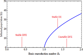
Figure 2. Forward bifurcation graph at  .
.
Download figure:
Standard image High-resolution image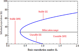
Figure 3. Backward bifurcation graph at  .
.
Download figure:
Standard image High-resolution imageNext, the conditions for the existence of an EE are derived and its stability behavior is discussed.
3.3. Investigation of the presence and local stability of the EE
This subsection investigates and discusses the local stability behavior of an equilibrium point of the system (3) for which the disease is endemic. By setting all equations of the system (3) to rest, i.e.,
We get,
where  is a solution to the following equation:

and,


Now, for  ,
,  is always negative and
  is positive. Thus, by Descartes's rule of signs [29], equation (8) has a unique positive value of
  for any
  . Hence, the following result is presented as a theorem for the existence of the unique positive EE:
Theorem 3. The system (3) always has a unique positive equilibrium  whenever
  .
.
Now, we discuss the local stability behavior of  .
.
For the local stability behavior of  , first, we obtain the corresponding linearized matrix
  of the system (3) at
  as given below:
The characteristic equation of the matrix  is
is

where

From equation (9), it is clear that one root is negative, i.e.  and the sign of other roots can be observed from the following quadratic equation:

In equation (10),  is always positive. Now, using the Routh–Hurwitz criterion, the following results are stated regarding the local stability behavior of
  in the form of two theorems.
Theorem 4. The endemic equilibrium  of the system (3) exhibits local asymptotical stability under the simultaneous conditions:
- (i),
- (ii)


Theorem 5. The endemic equilibrium  of the system (3) becomes unstable if any of the following conditions occur:
- (i);
- (ii);
- (iii) and


4. Global stability analysis
In this section, we focus on comprehending the global stability behavior of the EE. To achieve this goal, we assume that:
We now proceed to state and prove the following theorem regarding the global stability behavior of the EE:
Theorem 6. The endemic equilibrium  is globally asymptotically stable if
  .
.
Proof. At  , the following conditions are derived from the system (3):

Now, to establish the global stability of  , we define the Lyapunov function:

Differentiation of  along the solution of the system (3) is
After some arrangements, we have
Now, from the property of arithmetic mean, we have
and if
then,  . Hence, Using LaSalle's Invariance Principle [30], it can be deduced that if
  , the singleton set
  is the largest invariant set in
  and is globally asymptotically stable.
5.
Sensitivity analysis of the BRN

Sensitivity analysis of  helps to understand how uncertain the calculated value of
  is, and how much the outcome of the disease spread can be affected by parameter variations. To check the
  sensitivity, we calculate its derivatives as follows:
Because all parameters are positive, therefore,  and
and 
 . Thus,
  is increasing with p,
  and decreasing with
  .
.
6. Numerical results
In this section, system (3) is numerically simulated using Mathematica 11. The simulations are conducted using the numerically experimental parameter values listed in table 3.
Table 3. The parameter's numerical value.
| Parameter |

|

|

|

|

|

|

|

|

|

|
|---|---|---|---|---|---|---|---|---|---|---|
| Value |

|

|

|

|

|

|

|

|

|

|
The initial subpopulations are:

Using the dataset given in table 3, the EE  and the BRN
  are calculated as
  and
and  , respectively. Figure 4 illustrates the dynamics of the susceptible
  , infected
  , and hospitalized
  subpopulations when
  . It is evident from the figure that all subpopulations reach their endemic steady state,
  , over time. This observation confirms the local asymptotic stability result of the EE
  .
.
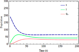
Figure 4. Subpopulations  with time.
Download figure:
Standard image High-resolution imageFigure 5 illustrates the number of infected individuals at various initial values of infected individuals  . The figure demonstrates that, regardless of the initial number of infected individuals, the infected population eventually reaches the same steady state. This observation confirms the global stability result of our study.

Figure 5. Infected population with higher  values.
Download figure:
Standard image High-resolution imageThe impact of the increased transmission rate  and inhibition rate
  on the infected population is illustrated in figures 6 and 7, respectively. As shown in figure 6, when the transmission rate rises, the number of infected individuals also increases. Conversely, figure 7 illustrates that as the inhibition rate increases, the number of infected individuals decreases. These findings suggest that controlling the spread of disease in society can be achieved by focusing on reducing the rate of infection transmission within the community and encouraging infected individuals to take necessary precautions.
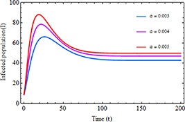
Figure 6. Infected population with the increased transmission rate  .
.
Download figure:
Standard image High-resolution image
Figure 7. Infected population with the increased inhibition rate  .
.
Download figure:
Standard image High-resolution imageThe impact of an increased hospitalization rate  and a limitation rate in hospitalization
  on the infected population is illustrated in figures 8 and 9, respectively. As depicted in figure 8, when the hospitalization rate increases, the number of infected individuals decreases. Conversely, figure 9 shows that as the limitation rate in hospitalization increases, the number of infected individuals also increases. These findings suggest that by enhancing the capacity to treat patients through measures such as adding hospital beds and increasing healthcare workers, doctors, and medical equipment, more infected individuals can receive treatment. This, in turn, reduces the risk of infection and lowers the number of fatalities in society.
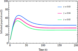
Figure 8. Infected population with the increased hospitalization rate  .
.
Download figure:
Standard image High-resolution image
Figure 9. Infected population with the increased rate of limitation in hospitalization  .
.
Download figure:
Standard image High-resolution imageFigures 10 and 11 demonstrate the impact of an increased hospitalization rate  and the limitation rate in hospitalization
  on the number of hospitalized individuals, respectively. As depicted in figure 10, as the value of
  increases, the number of infected individuals who are severely ill also rises. Conversely, figure 11 illustrates that by minimizing
  , more severely ill infected individuals can receive treatment in hospitals, which consequently leads to a notable improvement in the recovery of the infected population.

Figure 10. The hospitalized population with the increased hospitalization rate  .
.
Download figure:
Standard image High-resolution image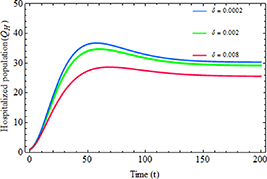
Figure 11. The hospitalized population with the increased rate of limitation in hospitalization  .
.
Download figure:
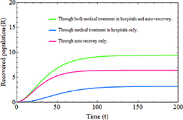
Standard image High-resolution imageFigure 12 illustrates the importance of incorporating the hospitalized population class into an epidemic model, especially concerning the number of individuals who have recovered from infection. The figure demonstrates that when the recovery of infected individuals through hospital treatment is considered alongside natural recovery, simultaneously, it results in a significantly greater increase in the total recovered population compared to considering a single recovery process such as relying solely on medical treatment or the auto-immune responses.
Figure 12. Recovered population over time.
Download figure:
Standard image High-resolution image
7. Discussion and conclusion
The goal of this study is to propose an epidemic model that includes a hospitalized class and analyze the stability behavior of the model. The incidence rate and hospitalization rate are modeled using the Holling type II functional form. Additionally, the BRN  is calculated using the next-generation matrix method. The paper concludes that the DFE is locally asymptotically stable if
  . This implies that the disease can be eradicated by maintaining the threshold parameter,
  , below unity. The center manifold theory is employed to analyze the model's behavior at
  . The analysis reveals that a forward (or backward) transcritical bifurcation occurs under specific conditions. Specifically, a forward transcritical bifurcation occurs when
  crosses unity from below, resulting in the emergence of a small, positive, asymptotically stable equilibrium. Conversely, a backward transcritical bifurcation occurs when
  . In this case, a small, positive unstable equilibrium appears alongside the locally asymptotically stable DFE and a stable larger positive equilibrium. From an epidemiological standpoint, a backward bifurcation implies that reducing the BRN to less than unity is insufficient to eliminate the disease. The paper also derives the conditions for the existence of the EE and demonstrates that the EE is locally asymptotically stable under certain conditions as stated in theorem (4), but unstable under others as given in theorem (5). Furthermore, the paper investigates the global stability of the EE and determines its global asymptotic stability under specific conditions when
  .
.
The theoretical findings of this study are strongly validated through numerical simulations. Figures 2 and 3 effectively illustrate the range and occurrence of forward and backward transcritical bifurcations in the model, utilizing the data from table 2. These simulations provide robust evidence, numerically validating both theorems 1 and 2. Figure 4 confirms the local asymptotical stability of the EE, as all subpopulations reach their respective steady states over time. Figure 5 is included to confirm the global stability result of the study. The evidence from figure 5 is clear: irrespective of the initial infected population, the system converges to the same equilibrium point. Moreover, the simulations demonstrate that adopting effective measures, such as wearing masks, regular hand sanitization, glove usage, hygiene maintenance, etc, by the population can significantly control the spread of infection. The importance of considering inhibitory effects is highlighted in figure 7. Furthermore, advocating for improvements in medical infrastructure allows severely infected individuals to access specialized treatment, resulting in more people receiving proper care, as depicted in figures 8 and 9. The significance of incorporating the 'Hospitalized' individuals class and considering a saturated hospitalization rate is demonstrated in figures 10 and 11, respectively. The importance of incorporation of hospitalized individual's class in the context of the increasing recovered population is also depicted in figure 12.
Beyond stability, the conclusion is that governments and health professionals should swiftly develop programs such as contact tracing and quarantine, while also ensuring an adequate number of spaces for quarantine. Additionally, ensuring the availability of medical infrastructure and adequate treatment facilities, including more hospitals, ventilators, and ICU beds, can help reduce the spread and accelerate the recovery of the infected population. These methods work to limit virus transmission and provide necessary care for the infected. Moreover, such programs should be sufficiently long-lasting to ensure the complete cessation of infection emergence. By increasing health education among individuals, developing a robust health infrastructure, and improving hospital facilities, we can effectively reduce the spread of infection and consequently decrease the loss of human lives. Health education plays a crucial role in increasing awareness and understanding of the virus and its transmission, leading to better compliance with measures such as contact tracing, quarantine, etc. This, in turn, helps alleviate the strain on healthcare systems during any epidemic outbreak.
Acknowledgments
The authors sincerely appreciate and thank the editors and anonymous referees for their invaluable comments and suggestions on the manuscript. The authors highly value their insightful feedback and helpful input, which significantly improved the manuscript's overall quality.
Data availability statement
All data that support the findings of this study are included within the article (and any supplementary files).
Funding
This work was not funded by any specific source.
Conflict of interest
The authors confirm no conflicts of interest.
Author contributions
All authors contributed equally to conceptualization, formal analysis, writing the original draft, and reviewing/editing of the manuscript.