
Abstract
Entropy has played an essential role in the history of physics. Its mathematical definition and applications have changed over time till today. In this paper, we first review the historical evolution of these various points of view, from the thermodynamic definition to information entropy from Shannon in classical physics, up to the modern concept of Neumann's quantum entropy. As a specific example, we consider entanglement entropy and compare the phase space approach in classical physics to the Hilbert space approach in quantum physics in simple model systems. We derive a general expression for the entanglement entropy of fermions and bosons in arbitrary partitions of Hilbert space, valid beyond the thermodynamic limit. Next, we compare thermodynamic heat engines with quantum heat engines. Finally, we proceed to the more general concept of quantum (computational) complexity and argue, using the concept of entanglement entropy, that the Heisenberg time in classically chaotic systems coincides with the time when maximal complexity is reached in the quantum case for systems with all–all interactions.
Export citation and abstract BibTeX RIS

Original content from this work may be used under the terms of the Creative Commons Attribution 4.0 licence. Any further distribution of this work must maintain attribution to the author(s) and the title of the work, journal citation and DOI.
1. Introduction
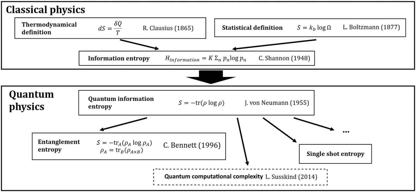
The concept of entropy has a long history, which dates back to the 19th century with the advent of thermodynamics. Till today, the concept has been generalized from classical to quantum physics in several steps, as shown in figure 1. Today, the concept of entanglement entropy plays an important role in modern quantum information theory (for a review, see reference [1]). However, also several other approaches and points of view concerning the concept of entropy, such as relations between single-shot state transitions in unitary quantum mechanics and the von Neumann entropy are part of an ongoing and inspiring discussion [2].

Figure 1. From classical to quantum entropy: information entropy (Shannon, 1948) can be viewed as the most general concept of entropy in classical physics. Its counterpart in quantum physics has been introduced by von Neumann 1955. Since that time, the concept of missing information in quantum physics has evolved in various manners. In this contribution, we focus mainly on the concept of entanglement entropy, and its relation to computational complexity as advocated by L Susskind in 2014.
Download figure:
Standard image High-resolution imageThe field of quantum physics along with its fascinating features and unique rules has altered our perspectives on the nature of matter substantially. The development of computers based on these features, so-called quantum computers or simulators, for example, has gained major interest in academia and industry alike and is in reach to be commercially utilized. Within the field of classical computation, a natural question to ask is that of the minimum number of simple operations required to carry out a given task, labeled computational complexity of a given task. This concept of computational complexity has been adopted and generalized by Susskind (2014) from classical computer science to the field of quantum computation/information theory. In this context, quantum computational complexity is defined as distance of a given quantum state |ψ⟩ from a given reference state |ψ0⟩ in terms of the minimal number of discrete computational steps to reach |ψ⟩ starting from |ψ0⟩. This question leads to a further extension of the concept of entanglement entropy, and to the extension of the second law of thermodynamics to the second law of complexity [3]. Note that this approach introduced by Susskind uses the term complexity in a much narrower sense than e.g. the complex-systems community [4]. In this contribution, we will only consider the aspect of quantum computational complexity.
Furthermore, we do not aim to provide a complete review on entropy and its usage in various disciplines. Rather, we put some spotlights on aspects of entropy from two different and complementing perspectives: from the perspective of physics education, we trace back some important aspects of the history of ideas related to entropy and its extension to complexity using simple models and calculations, focusing on key concepts. While the explicit model systems chosen in this contribution at first sight seem to be rather disjunct, we show that in all these cases, many if not all essential ingredients of the theory can be understood just from the simple properties of binomial distributions in various interpretations. In the thermodynamic limit, due to the central limit theorem, the details of the distribution becomes irrelevant. However, as discussed in section 4, our results for the mean entanglement entropy of fermionic and bosonic partitions remain valid even beyond this thermodynamic limit.
The second aim of our work is a thorough comparison of the concept of entropy in phase space defined by S = kB ln Ω, where Ω is the phase space volume, with the definition of entanglement entropy in the (reduced) Hilbert space  , i.e. S = kB trA
(ρA
ln ρA
), where ρA
= trB
ρ is the partial trace of the density matrix ρ of the Hilbert space
, i.e. S = kB trA
(ρA
ln ρA
), where ρA
= trB
ρ is the partial trace of the density matrix ρ of the Hilbert space  . We show that the number of Planck cells in Ω defines the dimension of the corresponding Hilbert space. In classical phase space, self-encounters of long periodic orbits within the same Planck cell play an essential role for the explanation of spectral correlations of classically chaotic quantum systems, [5, 6]. We compare this approach to the corresponding ansatz in Hilbert space, leading to nonlinear sigma models. Using the perspective of entanglement entropy, we show that the Heisenberg time is not only the time scale where the semi-classical phase transition emerges, and where orbits longer than the Heisenberg time cannot be resolved from shorter pseudo-orbits any more, but that the Heisenberg time coincides with the time scale where maximal complexity is reached for those quantum systems where all qubits do interact with each other.
This work is structured as follows: in section 2, we briefly review the definitions of entropy in classical thermodynamics (dS = δQ/T, R Clausius), in statistical physics (S = kB ln Ω, L Boltzmann) and in information theory (Hinf. = −K∑pk log pk ). In section 3, we extend these definitions to quantum physics, finally culminating in the concept of von Neumann's quantum entropy. As a specific application, we consider entanglement entropy (S = kB tr(ρA ln ρA ), C Bennett). Using some visualization ideas for mixed states introduced in references [7, 8], we explicitly find a relation between the definitions for entropy in phase space and in Hilbert space.
In the following three sections, we discuss applications of the concept of entropy in thermodynamics, statistical physics and in (quantum) information theory. We reverse the historical order in these sections, as the line of argument is easier when starting with the rather general concept of entanglement entropy: in section 3, we discuss dense coding in classical and in quantum physics using the simple binomial distributions in combination with the central limit theorem. In section 4, we discuss Planck's radiation formula in classical phase space, and translate it back to a simple binomial distribution in phase space. In Hilbert space, we show that this binomial defines the dimensions of the Hilbert space  and apply the concept of entanglement entropy both to photons and to a system of spins. These results remain valid beyond the thermodynamic limit, as long as quantum ergodicity (defined in (22)) can be assumed. In section 5, we discuss quantum heat engines using the system of spins introduced in section 4 including a time dynamics, which amounts to a time dependence in the binomial distribution of spins. As an explicit example, we derive the efficiency of a simple quantum heat engine, in analogy to the classical Otto cycle.
In section 6, we introduce and motivate the concept of (computational) complexity in a model of N qubits with all-all interaction: thermalization emerges at short time scales of the order of the Ehrenfest time, thus entropy becomes maximal at short time scales. On the other hand, we show that complexity grows for much longer time scales. By comparing the phase space with the Hilbert space approach, we argue that the Heisenberg time is the time scale of maximal complexity for a system where all qubits interact with each other, and discuss the relation to classical periodic orbits in phase space. This work ends with conclusions and an outlook in section 7.
2. Entropy in classical physics
Historically, the concept of entropy has been introduced phenomenologically by Rudolf Clausius in the beginning of the 19th century in the context of thermodynamics of heat engines. In modern notation, the thermodynamic definition of the change of entropy reads

where δQ is the heat exchanged between the heat reservoir and the working engine and T the associated temperature of the system. In 1877, Ludwig Boltzmann proposed a statistical definition of the entropy, which reads

where Ω counts the number of microstates in phase space leading to the same macrostate of the system, which in case of a heat engine corresponds to a gas of N particles in volume V with energy E. Since this time, within the framework of statistical physics, it is possible to relate the number of possible microscopic configurations and their probabilities to macroscopic observables based on explicit expressions for the entropy S = S(E, V, N).
It was only in 1948, that Claude Shannon published a seminal paper where he introduced the concept of entropy in a much broader context than thermodynamics. Consider a source that emits bit strings xk with probabilities pk . Then, the information entropy of an unknown bit string emitted by the source is given by

where K is a positive constant 4 . At first, Shannon called the function Hinf. 'missing information'. Only later, following a suggestion of von Neumann, the name information entropy was introduced.
Next, we discuss the important concept of maximal entropy. As pk
are probabilities, we first consider the maximum of H under the single constraint  for the microcanonical ensemble. Using the method of Lagrange multipliers, it is easy to see that pk
= const. = 1/N leads in this case to the maximum value K log N for the information entropy.
for the microcanonical ensemble. Using the method of Lagrange multipliers, it is easy to see that pk
= const. = 1/N leads in this case to the maximum value K log N for the information entropy.
In case of a (classical) Hamiltonian system, we introduce the expectation value for the inner energy  as an additional constraint for the canonical ensemble. The maximum value for Hinf. under these two constraints leads to
  . If we identify β−1 = kB
T and K → kB, (and changing the basis of the logarithm due to convention) we connect to the statistical definition of entropy of Boltzmann of equation (2), i.e.
. If we identify β−1 = kB
T and K → kB, (and changing the basis of the logarithm due to convention) we connect to the statistical definition of entropy of Boltzmann of equation (2), i.e.
to find the definition of the free energy F as

Thus, indeed the suggestion of von Neumann to call (3) entropy is justified and generalizes all previous concepts.
3. Entropy in quantum physics
Since missing information is at the heart of quantum physics, Shannon's information entropy (3) can directly be adopted to quantum states, when we view pk
as probabilities for quantum states |k⟩ in a mixed state. Let ρA
= ∑k
pk
|k⟩⟨k| be the density matrix describing the mixed state in Hilbert space  . Then, the quantum information entropy is given by

The last equality only holds if {|k⟩} are orthonormal. Note that for a pure state, the quantum information entropy is zero. Before plunging into applications, we first want to settle the history of ideas, finally leading to entanglement entropy [9, 10]. Entanglement entropy appeared for a pure state transformation by Bennett et al [11] in 1996, where the reversible transformation between multiple copies of maximally and non-maximally entangled bipartite states was considered.
The key idea is the following: any mixed state ρA
in Hilbert space  can be seen as a subset of a larger Hilbert space
  in a pure state ρA×B
with vanishing quantum information entropy. In this sense, the 'missing information' leading to information entropy is due to our ignorance of the full Hilbert space when tracing out the part B (the environment) to find the reduced density matrix ρA
= trB
ρA×B
. Note that by using the reduced density matrix (6), we find a function of probabilities, just as in the classical expressions for the entropies of equations (3) and (2). However, the interpretation has changed: while probabilities in classical physics are calculated in phase space, entanglement entropy is derived in Hilbert space. In Hilbert space, real probabilities are generalized and depend on complex amplitudes.
in a pure state ρA×B
with vanishing quantum information entropy. In this sense, the 'missing information' leading to information entropy is due to our ignorance of the full Hilbert space when tracing out the part B (the environment) to find the reduced density matrix ρA
= trB
ρA×B
. Note that by using the reduced density matrix (6), we find a function of probabilities, just as in the classical expressions for the entropies of equations (3) and (2). However, the interpretation has changed: while probabilities in classical physics are calculated in phase space, entanglement entropy is derived in Hilbert space. In Hilbert space, real probabilities are generalized and depend on complex amplitudes.
Let us illustrate the relation between the phase space and Hilbert space approach with the simplest possible example: a mixed system of a single qubit obtained from a pure system of two qubits by tracing out the 'environment', that is, a single qubit. A mixed state of a single qubit can be expressed as

where {|0a
⟩, |1a
⟩} denotes an orthonormal basis associated with  . Where we express the probabilities p0 and p1 in terms of the mixedness
  of the qubit. The mixedness
  can be visualized on the Bloch sphere S2 as shown in figure 2. In general, the quantum information entropy for a mixed single qubit with mixedness
  is given by equation (6) (setting K = 1),

Next, we seek to find an interpretation of the mixedness n in terms of the entanglement with a single qubit of the environment. In the standard |ij⟩-basis, the most general pure two-qubit state can be expressed as

with ∑ij
|zij
|2 = 1. Geometrically, these complex amplitudes correspond to the hypersphere S7. The degree of entanglement of the pure two-qubit state (9) can be expressed by the so-called concurrence
c = 2|z00
z11 − z01
z10| [12]. For c = 0, the qubits are independent of each other and |ψ⟩ is just given by a product state  in two independent Bloch-spheres S2 × S2. For c = 1, the qubits are the maximally entangled Bell-states and can be written as
  in any orthonormal basis set {|0b
⟩, |1b
⟩}. For an easy example, consider the full 22 × 22 density matrix
in any orthonormal basis set {|0b
⟩, |1b
⟩}. For an easy example, consider the full 22 × 22 density matrix  . Taking the partial trace of the first qubit A, we obtain the reduced density matrix

For the entanglement entropy, we find the same expression as in equation (8) with  . Thus, the probabilities p0, p1 in equation (7) can be derived from complex amplitudes in an extended Hilbert space. We conclude that entanglement with a second qubit can indeed be seen as the origin for the mixedness of a single qubit state.

Figure 2. Mixed states with different values for the mixedness  and probabilities p0 and p1, illustrated by the example of the states |0⟩, |1⟩.
Download figure:
Standard image High-resolution imageFor practical computations, it is much more convenient not to use the standard basis, but the so-called Schmidt decomposition: for a pure state, there exists a basis |ψ⟩ where its corresponding density matrix simply reads ρ4×4 = |ψ⟩⟨ψ|. Suppose we decompose the total Hilbert space as  , then the state |ψ⟩ can be expressed in the Schmidt decomposition as

with real values λj
fulfilling the normalization condition  . The entanglement entropy for the subsystem A is obtained by tracing out the environment B (or vice versa A), which leads to

From the Schmidt decomposition, it immediately follows that SA = SB . As obvious from equation (11), the original state is entangled unless λ1 or λ2 vanishes.
3.1. Entropy of entanglement as operational entanglement measure
The entropy of entanglement provides an operational entanglement measure, i.e., has an operational meaning for pure states. It gives the asymptotic conversion rates to maximally entangled qubit pairs  , and back. Consider n copies of a bipartite pure state |ψ⟩ shared between A and B with entropy of entanglements Sψ
. Then, one can find a sequence of local operations and classical communication—i.e., operations that act only on the qubits in A and the qubits in B, and A and B can communicate classically to share e.g. the results of measurements—that provide the transformations
, and back. Consider n copies of a bipartite pure state |ψ⟩ shared between A and B with entropy of entanglements Sψ
. Then, one can find a sequence of local operations and classical communication—i.e., operations that act only on the qubits in A and the qubits in B, and A and B can communicate classically to share e.g. the results of measurements—that provide the transformations  in the limit of large n. Notice that the transformations are approximate, but the error vanishes in the limit of n → ∞. So the entropy of entanglement tells us how many maximally entangled pairs one can generate from non-maximally entangled pairs, i.e. how useful the non-maximally entangled pairs are for applications such as teleportation (which requires one maximally entangled pair per teleportation). An entropy of Sψ
= 1/4 just means that n non-maximally entangled states |ψ⟩ contain the same amount of entanglement as n/4 maximally entangled pairs—and it is possible to extract this number of maximally entangled pairs. In turn, the reverse transformation is also possible. That is, the entropy of entanglement also provides the entanglement cost, i.e. the amount of entanglement that is required to prepare multiple copies of the non-maximally entangled states. Considering again Sψ
= 1/4, this means that n/4 maximally entangled pairs are necessary to prepare n copies of |ψ⟩ by local operations and classical communication only. The protocols are introduced and described in [11], further studied in [13].
in the limit of large n. Notice that the transformations are approximate, but the error vanishes in the limit of n → ∞. So the entropy of entanglement tells us how many maximally entangled pairs one can generate from non-maximally entangled pairs, i.e. how useful the non-maximally entangled pairs are for applications such as teleportation (which requires one maximally entangled pair per teleportation). An entropy of Sψ
= 1/4 just means that n non-maximally entangled states |ψ⟩ contain the same amount of entanglement as n/4 maximally entangled pairs—and it is possible to extract this number of maximally entangled pairs. In turn, the reverse transformation is also possible. That is, the entropy of entanglement also provides the entanglement cost, i.e. the amount of entanglement that is required to prepare multiple copies of the non-maximally entangled states. Considering again Sψ
= 1/4, this means that n/4 maximally entangled pairs are necessary to prepare n copies of |ψ⟩ by local operations and classical communication only. The protocols are introduced and described in [11], further studied in [13].
We also remark that for exact transformations between bipartite pure states, a single measure such as the entropy of entanglement does not suffice. Majorization criteria based on the Schmidt vectors of source and target state determine the possibility of a transformation [14], and its maximal success probability.
In case of mixed states, the situation is not so straightforward anymore. The mixedness of the reduced density operator of one system can result either from the fact that the two systems are entangled, or because the original overall state of the two systems has been mixed itself. Thus, the entropy of the reduced density operator is not directly related to the entanglement of the state [10].
3.2. Classical information entropy and Shannon's source coding theorem
Consider the simplest case of a classical source that produces a bit either with value 0 at probability p0, or 1 with probability p1. Since all classical information can be encoded in bits, the results derived here can easily be generalized. A random sequence of n such bits will be binomially distributed, i.e. the probability that a given sequence contains k1 ones and k0 = n − k1 zeros is given by  with p0 = 1 − p1, and there are binomial (n, k1) such bit strings with exactly k1 ones. Using Stirlings formula, we approximate the phase space partitions with k1 ones as

The binomial distribution is centered at  , see figure 3. This center of the Gaussian corresponds to the relevant part of the phase space, given by


Figure 3. In many applications, from all microstates in phase space (or the dimensions in Hilbert space, respectively) only a very small subset is relevant. Here, we show the decomposition of the phase space (Hilbert space) into parts where k = 0, 1, ...n of the bits (qubits) are '1', and (n − k) are zero. Each subspace contains n!/k!(n − k)! objects in phase space (dimensions in Hilbert space). Simply by replacing k by the expectation value ⟨k⟩ = np, we project to the relevant 2nS(p) microstates in phase space (subspace in Hilbert space), where S(p) is the entropy. Fluctuations become irrelevant in the thermodynamics limit n → ∞.
Download figure:
Standard image High-resolution imageFrom the fact that a binomial distribution approaches a Gaussian distribution in the large n limit, one sees that the bulk of the distribution lies in the interval  . Taking the neighboring k1s into account gives rise to a (vanishing) overhead, i.e. n(S(p1) + δ), where δ → 0. In this (thermodynamic) limit, all fluctuations become irrelevant, and only the peak value remains, drastically reducing the relevant phase space volume. The number of bit strings in this interval is of the order of
  , and labeling all these bit strings using nS(p1) bits provides a way to successfully transmit any of the possible sequences with vanishing error probability.
3.3. Noiseless quantum coding theorem
Similarly, as in classical information theory, entropy also plays a key role in quantum information theory. One of the earliest and nicest examples is the quantum version of the noiseless coding theorem put forward by B Schumacher [15]. For any given source of quantum systems described by a set of pure states with associated probabilities, {pj
, |ψj
⟩}, it provides the number of qubits that have to be transmitted to successfully relay a message of length n. The entropy of the source, i.e. the von Neumann entropy of the mixed state ρ = ∑j
pj
|ψj
⟩⟨ψj
|, Sρ
= −tr(ρ log ρ), gives the channel capacity. The transmission of n states from the source requires the transmission of nSρ
qubits. The basic idea behind the reduction is similar as for classical sources. However, in this case, not simply bit strings need to be transmitted as possible microstates in phase space, but whole subspaces in Hilbert space. The idea that the number of phase space cells in classical physics is generalized to the dimension of the Hilbert space will appear again in section 4.3. Consider first the case of the source producing orthogonal states, i.e. ⟨ψi
|ψj
⟩ = 0 whenever i ≠ j—and for simplicity also just two states |0⟩ and |1⟩ with probabilities p0 and p1, respectively. Following the same line of argumentation as in the classical case, there are likely sequences containing states of the form  with
with  (and permutations thereof). The basic idea is now to transmit the whole subspace spanned by all these basis vectors. The dimension of this subspace is
  as in the classical case, where we have used that the entropy of ρ coincides with the entropy of the classical probability distribution for orthogonal vectors. One can then show that submitting this subspace—which requires the transmission of nS(p1) qubits—suffices to successfully transmit the quantum information of all possible strings the source emits—with a vanishing error in the limit n → ∞.
An extension to non-orthogonal states, and a larger alphabet (or more possibilities) is straightforward. One has to look at the mixed state that describes the source, ρ = ∑j
pj
|ψj
⟩⟨ψj
|. One can use the spectral decomposition to write this mixed state in the form ρ = ∑k
λk
|k⟩⟨k|—and it turns out that the eigenvalues and eigenstates of the spectral decomposition characterize the source completely. Thus, it does not matter how a given density matrix is obtained or realized—as a mixture of non-orthogonal states, or by mixing eigenstates with probabilities specified by the eigenvalues. All sources that are described by the same density matrix are indistinguishable, and the same number of qubits is required to successfully transmit the information over a noiseless quantum channel. A successful transmission of quantum information produced by the source requires that an entangled state specified by a purification of ρ,  is preserved when one part of the state is transmitted through the quantum channel, and similarly for multiple copies. The probability distribution is a multinomial distribution rather than a binomial one as we treated in our example. However, there is still an expectation value for each of the basis states, given by
  . The multinomial distribution approaches a multi-dimensional Gaussian, and it is easy to see from the central limit theorem that the bulk of the distribution is contained around the expected values kj
≈ pj
n. So states of the form
. The multinomial distribution approaches a multi-dimensional Gaussian, and it is easy to see from the central limit theorem that the bulk of the distribution is contained around the expected values kj
≈ pj
n. So states of the form  with kj
≈ pj
n span the likely subspace, where multinomial coefficients describe how many states of this form exist (simply counting the number of permutations). From there, one can again determine the size of the likely subspace, which is given by 2nS(ρ) leading to the necessity to transmit n[S(ρ) + δ] qubits, where δ is some positive constant that determines the error probability. In the limit of large n → ∞, this is necessary and sufficient to guarantee a vanishing error probability for δ → 0.
with kj
≈ pj
n span the likely subspace, where multinomial coefficients describe how many states of this form exist (simply counting the number of permutations). From there, one can again determine the size of the likely subspace, which is given by 2nS(ρ) leading to the necessity to transmit n[S(ρ) + δ] qubits, where δ is some positive constant that determines the error probability. In the limit of large n → ∞, this is necessary and sufficient to guarantee a vanishing error probability for δ → 0.
Not surprisingly, entropies also appear in other problems of quantum information theory, in particular in quantum communication. We will only mention the important role of the Holevo quantity, quantum conditional entropy and quantum mutual information, but not go into further detail here (see reference [10] for an overview on the role of entropy in entanglement theory, [16] for an overview on quantum channel capacities, and [17] for an overview regarding entropic uncertainty relations, which express the inequivalence of several measurements performed on a quantum state and play an important role in the context of proving security of cryptographic protocols).
3.4. Entropy in entanglement purification protocols
Another interesting instance where entropies appear in quantum protocols are entanglement purification protocols. Entanglement is an important resource for various tasks in quantum information processing, e.g. to perform teleportation. However, pure state entanglement in the form of maximally entangled pairs is required, while due to the influence of noise, decoherence and imperfections, quantum states will typically be mixed and noisy. However, one can use several copies of a mixed state—which are e.g. generated by distributing them over some noisy channel—to distill fewer copies with higher fidelity. To this end, consider an ensemble of noisy entangled states of two qubits, where each pair is described by a density operator that is diagonal in the Bell basis |ϕj
⟩ = I ⊗ σj
|ϕ0⟩ with  . We thus have ρ = ∑j
λj
|ϕj
⟩⟨ϕj
| and Γ = ρ⊗n
, where λ0 = F is the fidelity of the state. The key idea is to view the ensemble as a mixture of all possible combinations of tensor products of Bell states with probabilities given by the coefficients λj
, where one lacks the information which of the configuration is present. In order to purify the ensemble and obtain multiple copies of maximally entangled pure states, one needs to figure out which of the configurations one is dealing with—i.e. one needs to learn the missing information. This is achieved by so-called random hashing, see reference [11].
. We thus have ρ = ∑j
λj
|ϕj
⟩⟨ϕj
| and Γ = ρ⊗n
, where λ0 = F is the fidelity of the state. The key idea is to view the ensemble as a mixture of all possible combinations of tensor products of Bell states with probabilities given by the coefficients λj
, where one lacks the information which of the configuration is present. In order to purify the ensemble and obtain multiple copies of maximally entangled pure states, one needs to figure out which of the configurations one is dealing with—i.e. one needs to learn the missing information. This is achieved by so-called random hashing, see reference [11].
In order to illustrate the basic idea, consider mixed states of rank 2, i.e. states with λ0 = F, λ1 = (1 − F) and λ2 = λ3 = 0. We refer to |ϕ0⟩ as the desired state, and to |ϕ1⟩ as the error state. We consider a bilateral CNOT operation, i.e. a controlled-X gate applied at party A and party B on two qubits. This is a local operation in the sense of the parties A and B, but joint operations on two copies. The action of this gate on two Bell pairs of the considered kind is as follows: |ϕi ⟩|ϕj ⟩ → |ϕi ⟩|ϕi⊕j ⟩. That is, information about the error in the first entangled pair is transferred to the second entangled pair. By using such a bilateral CNOT gate with several different pairs as source, and always the same pair as target, the target pair actually shows the parity information about the total number of error states in this sub-ensemble. This parity information, i.e. whether one has an even or odd number of errors in the whole considered sub-ensemble, can be read out by performing local Z measurements on the qubits of the target pair, and classically communicating the results. If the measurement results coincide, there was an even number of errors, if not, the number of errors is odd. Notice that the entanglement in the target pair is destroyed by the measurement, i.e. the pair is consumed, but one bit of information on the sub-ensemble is revealed. We will use this as a tool to learn the desired information about a bigger ensemble, and determine the actual configuration of error states, i.e. the number of error states and their position. Once this is known, the ensemble is actually purified, as one then knows which of the possible configurations is present, and one can correct error states to the desired ones by applying a σx operation on the qubit in B. It is actually sufficient to measure the parity information on the number of error states in randomly selected sub-ensembles, as from sufficiently many such measurements the distribution of the error states can be determined. Each of the measurements reveal one bit of information, and for large ensembles and randomly selected sub-ensembles, these bits are independent [11].
It remains to show how much information is required, i.e. how many pairs of the ensemble need to be measured. For this, we can again use the insight on likely sequences and likely subspaces discussed in the context of the noisy (quantum) coding theorem. The mixed state ρ⊗n
can be seen as a mixture of states of the form  with k0 + k1 = n, with corresponding probability
  , and there are binomial (n, k1) permutations of this kind. The probability distribution is centered around
  ,
,  , where the neighborhood correspond to the likely configurations. Assuming for simplicity that the number of error states is exactly
  , there are
  configurations of this kind, and one needs nS(λ0, λ1) bits of information to reveal which of the configurations is present. Further taking the neighboring configurations
  into account leads to a small correction nδ. Hence by measuring n[S(λ0, λ1) + δ] pairs, one can determine which of the configuration is present, thereby purifying the remaining ensemble of n[1 − S(λ0, λ1) − δ] pairs. A similar analysis holds true for general Bell-diagonal states.
This entanglement distillation protocol is optimal for the discussed rank-2 states, but not for general rank-4 states. Further details can be found in reference [18]. Nevertheless, it is interesting to see that the same concept of likely sequences and subspaces, which rely on the simple combination of multinomials and the central limit theorem as illustrated in figure 3, shows up again in a broader context.
4. Oscillator models in phase space and in Hilbert space
4.1. Planck's radiation formula in phase space
Next, we want to show that binomial distributions are also a key ingredient for the historically important derivation of Planck's radiation formula and its generalization in the framework of entanglement entropy. In 1900, Max Planck derived his famous formula describing black-body radiation using a simple oscillator model using the concept of classical phase space. In this section, we review and extend this model and compare phase space and Hilbert space approach.
Consider P different oscillators, among which N energy portions  are randomly distributed. The energy portion is proportional to the associated oscillator frequency, i.e. ∝ ν. In order to fit with the experiment, Planck empirically found

This equation can be understood as an expression for the temperature T = T(E) as a function of energy. Using some kind of mathematical reengineering, he derived from ∂S/∂E = 1/T(E) an expression for the entropy of the black-body radiation at temperature T = T(E) by integration of the empirical result (15), leading to
meaning that the total number of microstates of the black-body radiation at temperature T within the oscillator model is larger than the usual value ΩBoltzmann = PN
/N! from the Boltzmann statistics. When Planck derived the entropy (15) from the experimental data of the black-body radiation, the interpretation was not clear yet. In particular, the fundamental meaning of the proportionality constant in = hν had not been settled yet.
4.2. Counting Planck cells in phase space space
Quantum physics provides an interesting interpretation of Planck's constant h as the smallest countable unit in phase space. The classical phase space Ω(E, N, V) is thus divided into a discrete set of P 'Planck cells' with P = Ω(E, N, V)/(2πℏ)3N in phase space 5 .
Now, suppose that N energy quanta will be filled into these P Planck cells. Then, we can distinguish three physically relevant expressions for the number of possible microstates:
Indeed, repeating the steps shown after equation (15) for the black-body radiation, using Stirlings formula, we recover Fermi–Dirac statistics, Boltzmann statistics, and Bose–Einstein-statistics from these binomial distributions.
The subtle statistical differences between fermions, bosons, and the classical Boltzmann statistics can be read off from (17) as follows: in case of Boltzmann statistics, the energy quanta have no influence on each other. For fermions, each Planck cell may only be occupied at most once. Thus, the first energy quantum has P choices, the second (P − 1), and so on. As the energy quanta are indistinguishable for a given energy, we must divide by 1/N!, leading to P(P − 1)(P − 2)...(P − N + 1)/N! microstates. This is the well-known interpretation of Pauli's principle in Hilbert space, leading to antibunching.
For bosons, the reverse is true: the first energy quantum again has P choices, but in contrast to fermions, subsequent bosons have not less, but more choices: the second qubit has (P + 1), the third (P + 2), and so on. In the ansatz of Einstein [19], this statistical behavior is called stimulated emission: bosons of the same energy and in the same phase space cell stimulate each other, which is expressed by a larger phase space volume. The number of bosons that may occupy the same phase space cell is unlimited, and a given energy quantum in a cell increases the probability for the next quantum to occupy the same cell. This behavior is called bunching.
We may ask which of these two key ideas—Pauli's principle or stimulated emission—can be derived from more general principles. In both cases, experimental data has been the starting point for the statistical expression given by (17), and in both cases, up to know, the quest for 'deeper' or more fundamental reasons for this behavior are a topic of active research.
Note that the definition of a temperature as a statistical property is only possible in the thermodynamic limit, where Stirlings approximation in (17) can be applied. However, the statistics for bosons and fermions as described by the binomials in (17) remains valid also beyond this thermodynamic limit. We will discuss this point further in the following section, when proceeding to entanglement entropy in Hilbert space.
4.3. Entanglement entropy approach in Hilbert space
Classical entropy is defined in phase space, while quantum entropy is a function of amplitudes in an extended Hilbert space. At first, these two approaches seem to be very different. Here, we want to show how the concept of entanglement entropy can provide a unified viewpoint for both approaches.
Consider N spins of a paramagnet with Hamiltonian  in Hilbert space. Suppose that on average, n1 spins are parallel, and n2 antiparallel to the magnetic field at given temperature T. The total energy is then given by
  , and the mean energy per spin is given by
  . Then, the phase space volume reads

From this expression, we can derive the probability for spin up/down with respect to the direction of the magnetic field as  with β = 1/(kB
T). As the degree of freedom of spin is defined in Hilbert space, at first, this problem looks quite different as compared to degrees of freedom in phase space. Since no phase space description is available, the spin is sometimes considered to be prototypical for quantum physics. However, we will show in what follows, that this is not the case, as the description in phase space can also be generalized using entanglement entropy in an extended Hilbert space for bosonic systems. In this sense, the spin system is nothing special.
with β = 1/(kB
T). As the degree of freedom of spin is defined in Hilbert space, at first, this problem looks quite different as compared to degrees of freedom in phase space. Since no phase space description is available, the spin is sometimes considered to be prototypical for quantum physics. However, we will show in what follows, that this is not the case, as the description in phase space can also be generalized using entanglement entropy in an extended Hilbert space for bosonic systems. In this sense, the spin system is nothing special.
While the Hamiltonian  does not include interactions between the spins, the mere fact that the spins share the same temperature necessarily includes thermalization due to interaction with a heat bath. Whatever small this interaction might be, any such incoherent interaction leads to entanglement with the environment. Thus, we may view the mixed state ρ = pup|0⟩⟨0| + pdown|1⟩⟨1| with entropy (8) in Hilbert space
  as a result of entanglement with the environment in the extended Hilbert space
  . More in general, as shown in figure 4, we may divide the spin system with N = NA
+ NB
spins into two subsystems A, B. For the number of possible microstates in each subsystem A, B, we obtain
. More in general, as shown in figure 4, we may divide the spin system with N = NA
+ NB
spins into two subsystems A, B. For the number of possible microstates in each subsystem A, B, we obtain
Thus, the Hilbert space is divided into a direct sum of the type

where dE
is the dimension is the full Hilbert space, and dj
= Hj
(j
) the dimension of a particular partition. How can we calculate the entanglement entropy for this system? The number of microstates dA/B
(nA/B
) defines the dimension of the Hilbert spaces  . Indeed, there are dA/B
(nA/B
) states composed from nA/B
qubits |0⟩ and N − nA/B
qubits |1⟩. We label these states as |ai
⟩ and |bk
⟩, with i = 1, ...dA
(nA
) and k = 1, ...dB
(nB
). Similar as in (9), we express a pure state of the composite system as
. Indeed, there are dA/B
(nA/B
) states composed from nA/B
qubits |0⟩ and N − nA/B
qubits |1⟩. We label these states as |ai
⟩ and |bk
⟩, with i = 1, ...dA
(nA
) and k = 1, ...dB
(nB
). Similar as in (9), we express a pure state of the composite system as
The entanglement entropy for a particular configuration described by the amplitudes zik is then obtained by tracing out the environment ρA ≡ trB (ρA×B ) and calculating SA (zik ) = −trA (ρA log ρA ). Unitary time development in the full Hilbert space leads to time-dependent amplitudes zik (t), and in turn to a time-dependent entanglement entropy, which can be calculated from the specific Hamiltonian of the system. We assume that time development leads to quantum ergodicity in Hilbert space if all degrees of freedom do interact uniformly with each other. Numerically, it can be shown in simple model systems with all-all interaction that a very small number of qubits is sufficient to reach this limit. Then, the entropy of entanglement converges to the mean value obtained by integrating over the full Hilbert space with equal measure

Note the analogy to the approach in phase space: also in phase space, the time development of the coordinates (x(t), p(t)) derived from the classical Hamiltonian in case of a fully chaotic system can be replaced by a phase space integral dp dx under the assumption of ergodicity.

Figure 4. (a) Visualization of a random spin partition A, B of a spin system. (b) Visualization of a random partition of P Planck cells occupied by N energy quanta into partitions A, B. In the bosonic case, the N energy quanta which are already present increase the number of possibilities, see (26). In the fermionic case, each Planck cell can only be occupied once as in the case of the spin system (19). In case of the Maxwell–Boltzmann statistics, the energy quanta do not influence each other at all, see (27).
Download figure:
Standard image High-resolution imageThe integral in Hilbert space can be calculated using random matrix theory as shown in reference [20]. The result is the celebrated Page formula for the mean entanglement entropy in Hilbert space  , which is an analytic and exact result, depending only on the dimensions
dA
and dB
of
, which is an analytic and exact result, depending only on the dimensions
dA
and dB
of  [21]
[21]

where Ψ(x) = Γ'(x)/Γ(x) is the logarithmic derivative of the gamma function Γ(x). In the limit of large heat bath (dB ≫ dA ), we obtain the approximation

It follows that the typical entropy of entanglement is close to the maximum value. For an environment B with k qubits, the corrections fade out as  .
.
When we divide our system of N spins with n1 spins 'up' into parts A and B, in order to obtain the mean entanglement entropy, there is one more technical step to be considered: the Page equation holds true for one partition with  as shown in equation (20). Summing up all partitions, the exact result for the full mean entropy has been calculated analytically in references [20, 21] as

The entanglement entropy only depends on the dimensions of the Hilbert spaces in each partition. For the spin system, these partitions are given by equation (19). In case of a Bose gas, we find partitions of type
with N = NA + NB , P = PA + PB and where P is the number Planck cells in phase space, and N number of bosons. For fermions, the partitions are given by (19) while for the Boltzmann statistics, the partitions read

In all these cases, the mean entanglement entropy (25) reproduces the results for the entropy obtained in phase space in the limit of a large environment PB . For example, in the spin system, we obtain for a large total number of spins N [20]

with  with n ≡ n1 − n2. Again, only a very small subspace of the Hilbert space (20) finally turns out to be relevant, and again the argument boils down just to restrict to expectation values of binomial distributions as in equation (14).
Note that the derivation and definition of temperature from entanglement entropy is only possible for NA ≪ N, as only in this (thermodynamic) limit, the usual arguments of statistical mechanics allowing to ignore fluctuations of the entropy can be applied. Exact (and rather involved) expressions for the fluctuations of the entropy of entanglement have been derived in [20]. The fluctuations for a given partition can be approximated by

for dB ≫ 1 and indeed fade out in the thermodynamic limit [20] as 1/dB . Only in this limit, a temperature can be defined in the sense of thermodynamics. However, the partitions (19) and (26) are valid beyond this thermodynamic limit. Under the assumption of quantum ergodicity, that is, integrating the whole Hilbert space with uniform measure as defined in (22), using the exact expressions for the entanglement entropy (23) and (25) and the pertinent expressions for fluctuations from the mean entropy [20], quantum corrections to the thermodynamics of fermions and boson can be discussed for NA ≃ NB and for very small system sizes.
To summarize, we have shown that the entropy of entanglement provides a unified viewpoint for physical systems in Hilbert space even beyond the thermodynamic limit. The number of relevant Planck cells in phase space defines the dimension of pertinent Hilbert space. Note that this is a simple counting argument, which, much the same as Weyl's law [6], does not make any assumptions concerning the localization of eigenfunctions of the pertinent Hamiltonian within the Hilbert space.
5. Quantum heat engines
5.1. Thermodynamic definition of entropy and heat engines
Next, we consider quantum thermodynamic heat engines (QHEs) (in the limit NA ≪ N) that—in analogy to classical heat engines—produce power by transferring heat from a hot into a cold heat reservoir. Such (quantum) thermodynamic cycles reveal a cornerstone in modern physics and have substantially changed human's life since the first industrial revolution in the 19th century.
The central model used in this historical context is that of an ideal gas of N particles confined in a box of volume V and with kinetic energy  . Then, the phase space volume

leads to the entropy of the ideal gas

with U = ⟨E⟩. For a fixed number of particles, the change of entropy reads

With  , and pV = NkB
T this expression is equivalent to dU = T dS − p dV. Comparing this with the first law of thermodynamics dU = δQ + δW, we arrive at the expression of Clausius for the change of entropy
, and pV = NkB
T this expression is equivalent to dU = T dS − p dV. Comparing this with the first law of thermodynamics dU = δQ + δW, we arrive at the expression of Clausius for the change of entropy  which is the starting point to describe heat engines, e.g. the Otto cycle. Within classical physics, these results do not change if we divide the volume V into small but constant subvolumes V0. We may read B = V/V0 as number of possible regions where N particles can be arranged, which would again lead to ΩBoltzmann = BN
/N! as discussed in the previous section. In 1905, Einstein used this analogy to the ideal gas in configuration space in his first attempts to describe the statistics of photons starting from Wien's law.
which is the starting point to describe heat engines, e.g. the Otto cycle. Within classical physics, these results do not change if we divide the volume V into small but constant subvolumes V0. We may read B = V/V0 as number of possible regions where N particles can be arranged, which would again lead to ΩBoltzmann = BN
/N! as discussed in the previous section. In 1905, Einstein used this analogy to the ideal gas in configuration space in his first attempts to describe the statistics of photons starting from Wien's law.
In what follows, we will discuss the few-particle regime (NA ≃ 1), where quantum effects take place and whose theoretical [22, 23] investigation has opened an active, current research direction. Recent experiments on quantum heat engines based on a single qubit could be successfully implemented using various setups [24–29]. In this field, the thermodynamic definition of entropy, dS = dQ/T of equation (30), plays a crucial role to describe the properties of the thermodynamic system of interest. Note that for the definition of the temperature and ignoring fluctuations, the heat bath must be much larger than the system size (NA ≪ N). An illustration of such a quantum Otto cycle [30, 31] can be found in figure 5.

Figure 5. Thermodynamic entropy—working parameter diagram of quantum Otto cycle. The quantum Otto cycle has two isentropic work-exchange (1 and 3) and two isochoric heat-exchange strokes (2 and 4) in which the working medium (WM) is alternating coupled to an environment that is illustrated as two heat baths at cold Tc and hot temperature Th.
Download figure:
Standard image High-resolution image5.2. Entanglement entropy in the framework of quantum heat engines
In analogy to classical heat engines, its quantum version also consists of four strokes: in the two isentropic strokes (1 and 3) the quantum WM, e.g. a quantum harmonic oscillator, or an electron's spin, exchanges work with an environment by being 'compressed' and 'expanded' by changing the working parameter λ, which is in our example the magnetic field strength. During the isentropic strokes, the dynamics are considered to describe an isolated system where no heat is exchanged with the environment, thus keeping its entropy constant.
In the two heat-exchange strokes, the WM is alternating coupled to two heat reservoirs at cold Tc and hot temperature Th, respectively. Thus, the WM exchanges heat with the environment until it reaches thermal equilibrium, where the entropy flows in the same direction as the heat.
For our illustration, we choose a quantum WM that consists of a single spin and which can be parametrized by the state Hamiltonian

where the magnetic field acts as a 'working parameter', i.e. B ∝ λ (figure 5). We assume that the magnetic field varies linearly between a small value Bc and a large value Bh. The energy splitting thus varies between c ≡ μBc for the points A, D and h ≡ μBh > c for B, C of the quantum Otto cycle of figure 5. The entanglement entropy of the single spin is given by equation (28) with NA
= 1, thus

where the probabilities p± to find the spin values ± are then given by ![${p}_{\pm }=\frac{1}{2}\left\{1\pm \mathrm{tanh}[\beta (t){\epsilon}(t)]\right\}=\frac{1}{2}\left(1\pm E/{\epsilon}(t)\right]$](https://content.cld.iop.org/journals/1751-8121/55/40/404006/revision2/aac8f74ieqn57.gif) . Here, E = tr(ρH) is the expectation value for the energy.
. Here, E = tr(ρH) is the expectation value for the energy.
The strokes of the quantum Otto cycle read as follows:
- (a)Isentropic 'compression' (A → B): in A, the spin is in its thermal equilibrium state at temperature TA = Tc. The 'compression' for the quantum Otto cycle is achieved by increasing the magnetic field and thus the energy splitting fromc to h. The isentropic stroke can be described as a sequence of quasi-static unitary transformations and thus no heat is exchanged with the environment. In analogy to the compression stroke of a classical Otto cycle, the entropy remains constant and in turn the probabilities for spin up/down as defined by the binomial distribution in (14) and (33). The mixedness of the qubit remains fixed, while the energy splitting increases with constant β.
- (b)Isochoric heating: (B → C): in B, the spin is not in thermal equilibrium anymore. The temperature TB is given by TB = (h/c)TA
. The WM is brought in contact with the hot reservoir at temperature Th. While the energy splitting remains constant, the probabilities for spin up/down as defined in (14) and (33) change and in turn the mixedness of the qubit and the entropy, until thermalization is achieved. During this heat-exchange stroke, the heat
 as the difference in energy between the points B and C is imparted by the hot reservoir into the cold. The duration of this isochoric stroke is in general much shorter than the isentropic stroke due to the requirement on quantum adiabaticity (see below).
 - (c)Isentropic 'expansion' (C → D): in C, the spin is in its thermal equilibrium state at temperature TC = Th. During this 'power stroke', the WM exchanges the work while the magnetic field quantum adiabatically decreases. While the energy splitting decreases, much the same as during the isentropic 'compression', the mixedness of the qubit remains fixed, and in turn β.
- (d)Isochoric cooling: (D → A): in D, similar as to (b), the spin is not in thermal equilibrium anymore. The temperature TD is given by TD = (c/h)TC
. The WM is brought in contact with the cold reservoir at temperature Tc until it thermalizes back into its original initial thermal state ρA
. During this 'cooling' stroke, the heat as the energy difference between the points A and D is transferred into the cold reservoir, consequently decreasing the entropy.


In analogy to their classical counterpart, we can find an appropriate expression for the efficiency of such quantum heat engines, defined as the useful work divided by the heat  imparted by the hot bath, i.e.

For the quantum Otto cycle of figure 5, we find

In analogy to classical Otto heat engines, the ratio of energy splittings c/h due to the oscillating magnetic field can be regarded as the 'compression coefficient'. A detailed derivation of the efficiency η (35) can be found in appendix
Such quantum thermodynamic cycles depict an irreversible process in which, according to the second law of (quantum) thermodynamics, the thermodynamic entropy Sirr. ⩾ 0 of the whole composite system AB, consisting of the quantum Otto cycle (subsystem A) and the environment (subsystem B), increases. In such thermodynamic processes, the notion of entropy can be viewed as a measure of irreversibility, that is, 'closing' the cycle by getting back to the initial point A of figure 5 usually requires an irreversible change in the environment which manifests itself as flown heat Q.
Although the strokes and working mechanisms of the quantum Otto cycle look very similar to its classical analog, there exists a fundamental difference between the former and the latter. Whereas in the classical case, the adiabatic work-exchange strokes require no heat transfer due to a fast stroke—such that the latter remains quasi-static and the system does not have time to get out-of-equilibrium—the same, however, is not true in the quantum case. Here, the work-exchange strokes are adiabatic in a quantum sense, that is, they are so slow such that the system remains in its instantaneous eigenstate during the whole isentropic stroke, thus keeping their populations constant during the latter. This feature constitutes a severe hindrance in the development of efficient quantum heat engines that operate at finite time while still producing a high power output and efficiency and has been object of current research [32–36].
In such finite-time quantum heat engines and refrigerators, the excitation of coherences in the work-exchange causes the system to be driven out-of-equilibrium. The information on these excitations, that are stored in the off-diagonal elements of the corresponding density matrix, are dissipated away in the heat-exchange strokes. The latter feature is analogous to classical mechanics and has been dubbed quantum friction [37–39] and which is equivalent to an increase in the thermodynamic entropy, equation (30), of the composite system. In a nutshell, this increase in the thermodynamic entropy can be calculated from the change of probabilities for spin up/down using the time dependent binomial distribution in (14) and (33) for the four steps (a)–(d) of the cycle.
As a future work, using the ansatz described in section 4.3, it would be interesting to shrink the size of the heat bath beyond the thermodynamic limit with only a few qubits NB , such that fluctuations of the entropy cannot be neglected anymore.
6. Time scales in phase space and Hilbert space—from entropy to complexity
In the previous sections, we discussed applications of the concept of (entanglement) entropy both in classical and in quantum physics in simple examples, emphasizing the relation between the number of Planck cells in phase space and the dimension of the corresponding Hilbert space.
This comparison of the phase space and the Hilbert space approach is fruitful in many aspects. In phase space, semi-classical techniques can be applied for explicit calculations, while in Hilbert space, quantum field theory is at hand. In particular, for classically chaotic systems, the importance of self-encounters of long classical orbits in phase space has been established, e.g. to explain spectral correlations [5, 6]. Within a self-encounter, two parts of a long periodic orbit come as close as ℏ in phase space, that is, visit the same phase space cell. After the Ehrenfest time tE defined by  (where λ is the Lyapunov-exponent of the orbit and c is a constant), the self-encounter ends and the two orbits' stretches are again far apart from each other. Correlations between classical orbits that lead to a quantum signature of chaos originate from the fact that within the encounter region, reconnections between the orbit stretches again lead to classical solutions for partner orbits which differ from the original orbit only within the encounter region, with action difference of the order of ℏ [5]. Compared to the Hilbert space approach, a one-to-one correspondence between perturbative expansions within the formalism of nonlinear sigma models and a semi-classical theory using encounters of pairs of classical periodic orbits pairs has been established. Using these techniques, results from random matrix theory can be reproduced using periodic orbit theory in phase space, leading to a semi-classical understanding for the origin of spectral correlations in terms of correlations between periodic orbits for classically chaotic systems [40].
In recent time, this approach has been generalized to many body systems [41], and in particular, a close relation between entanglement and encounters has been established. The maximal entanglement entropy is reached at a time scale of the order of the Ehrenfest time, also known as scrambling time in the context of quantum gravity. While thermalization is a fast process, the time scale to resolve the complete spectrum is much larger. Let us choose a system of N qubits with all–all interaction as an explicit example. For such a quantum circuit with N qubits, it is sufficient to introduce e.g. single-qubit and CNOT-gates as simple operations as an exactly universal gate set [42].
The dimension of the Hilbert space is 2N = eNln 2 = eS , corresponding to the number of Planck cells in phase space, and according to Weyl law, to the number of energy levels for classically chaotic systems. Almost all states have maximal entropy S = N log 2, and the mean level spacing fulfills Δ ∝ e−S . The time needed to resolve the mean level spacing is given by the Heisenberg time defined by tHΔ ≃ ℏ. Thus tH = ℏ/Δ ∝ eS ≫ tE [43].
The scrambling time for this case is given by tE ∝ log N, thus in this model N−1 ∝ heff. Here, we derive this relation using an ansatz inspired by percolation theory. Starting with an arbitrary qubit, how many time steps are needed with single qubit–qubit interactions, such that this qubit in connected by a chain of interactions to all other qubits? As shown in figure 6, in each time step Δτ ≡ λ−1, all N qubits do interact, such that there are g = N/2 CNOT-gates. We consider the (arbitrary) 'first' qubit, which interacts with one other qubit. After the first step k = 0, δgl = 1 gates are 'linked' to the first gate. Thus the probability that a given qubit is linked to the first at k = 0 is given by p1 = 1/(N − 1) ≃ 1/N. In step k, there are gl gates 'linked' to the first gate. Let pl (k) = 2gl /N be the probability that a given qubit is 'linked' to the first qubit after k steps. In the next time step, this probability changes by

In the continuum limit, we find with the initial condition pl (0) = 1/(N − 1)

with scrambling time tscr. ≃ 1/λ ln(N) for large N. A similar result has been obtained by Kitaev for Majorana fermions [44]. In the context of quantum chaos, this time scale is also known as Ehrenfest time. Note that all–all interactions are necessary for the derivation of the ln(N)-dependence. In contrast, in Ising-like models only with nearest neighbor interactions, a polynomial N-dependence is found.

Figure 6. Quantum circuit of N qubits: in each time step, N/2 two-qubit operations are performed. In this model, all qubits do interact with each other. There are (N − 1)!! different possible combinations of pairs of two-qubit interactions. While thermalization is achieved after the Ehrenfest time tE ∝ log N, complexity grows for a much longer time scale and reaches its maximum after the Heisenberg time tH ∝ 2N .
Download figure:
Standard image High-resolution image
While entropy does not grow anymore after the Ehrenfest time, in recent time, the concept of quantum computational complexity as introduced by Susskind has attracted much interest, as generalization of the concept of entanglement entropy [3]. Note that in this context, the term quantum computational complexity is used here a much narrower meaning than in the complex-systems community [4].
Computational complexity answers the question: what is the minimum number of simple operations needed to reach a certain computational goal? In classical physics, at least k1 bit-flip operations are needed to reach a classical n-bit string within the partition containing k1 ones starting from the N-bit string {000, ...}. The order of magnitude of the information entropy of this ensemble of bit strings coincides with that of computational complexity, compare equation (13).
However, in quantum physics, there is a dramatic difference [3]. Quantum computational complexity is defined as the minimal number of gates needed to change from an initial state |ψ0⟩ to a target state |ψT⟩. For our argument, it is sufficient just to consider two-qubit operations as shown in figure 6. In each computational step, we assume that all N qubits do interact in a set of pairs with each other. Then, there are d = (N − 1)!! possible combinations of two-qubit operations to find pairs of N qubits. To leading order, we approximate these possible combinations as d = N!/[2N/2(N/2)!] ≃ NN/2. After k time steps,  of these possibilities have been explored, see figure 6. Thus, the complexity
  of the circuit grows linearly with the number of time steps as
  . While the entropy is maximal already after the Ehrenfest time, the complexity still grows for a very long time, which has been proposed as the second law of complexity by Susskind [45]. The time behaviour of complexity has been studied analytically and numerically in various systems [46]. It turns out that quantum ergodicity, that is, a system where all qubits do interact with all others (in contrast, e.g. to nearest-neighbour interaction), is necessary to reach maximal complexity. This corresponds to a fully chaotic phase space (in contrast, e.g. to mixed phase space). In this case, the complexity grows for long times, however, it becomes maximal after k ∝ eS
time steps, that is, after the Heisenberg time.
. While the entropy is maximal already after the Ehrenfest time, the complexity still grows for a very long time, which has been proposed as the second law of complexity by Susskind [45]. The time behaviour of complexity has been studied analytically and numerically in various systems [46]. It turns out that quantum ergodicity, that is, a system where all qubits do interact with all others (in contrast, e.g. to nearest-neighbour interaction), is necessary to reach maximal complexity. This corresponds to a fully chaotic phase space (in contrast, e.g. to mixed phase space). In this case, the complexity grows for long times, however, it becomes maximal after k ∝ eS
time steps, that is, after the Heisenberg time.
A similar behavior can be found for spectral the form factor. To see this, it is fruitful to compare the underlying mechanisms in phase space and in Hilbert space: concerning periodic orbits, within the resolution of phase space given by the size of Planck cells ℏ, orbits of lengths larger than the Heisenberg time can effectively be seen as composed of a combination of shorter pseudo-orbits, reconnected within encounter regions. Since all shorter orbits share at least one encounter region with any orbit of length larger than the Heisenberg time, all longer orbits can be rewritten as a combination of these pseudo-orbits within the course-grained resolution of ℏ in phase space. In this sense, nothing 'new' happens after Heisenberg time, as any longer orbit can be viewed as a repetition of shorter pseudo orbits glued together in encounter regions. In such a way, the one-to-one correspondence between a perturbative expansion in the nonlinear sigma model and the semi-classical approach using pairs of classical pseudo-orbits pairs can be extended beyond the Heisenberg time [47].
Technically, in the Hilbert space description of random matrix theory, we again meet a similar idea as those shown in figure 3. The maximum of the binomial distribution is the only relevant part of Hilbert space for dense coding, thus within the vast Hilbert space, only a very small subset remains important, which is the saddle point of the probability distribution. Within the nonlinear sigma model, in a similar manner, the integral over the full Hilbert space with random matrices is replaced using a colour-flavor transformation by an integral over saddle point manifolds, which again leads to a drastic reduction of dimension. While the short-time behavior (smaller than the Heisenberg-time) is described by the perturbative expansion around the standard-saddle point manifold, the longtime contribution (larger than the Heisenberg-time) comes from the so-called Altschuler–Andreev saddle point manifold.
Concerning complexity, it is striking that there is a close analogy in the argument: we introduce an approximate complexity  defined as the minimum number of gates in V to approximate the given unitary operator U such that ||U − V|| ⩽ . Thus, within the resolution of -balls in Hilbert space, there is a finite number
  of effectively distinguishable gate combinations, given by the number of such -balls in Hilbert space. In leading order,
  [45], for systems of qubits where any kind of two-qubit interaction is present, with only a weak dependence on the size of the -balls. In [46], this result is shown for abelian gauge theories in case that the interaction is maximally nonlocal. Since all
-balls in Hilbert space have been visited after the Heisenberg time, the repertoire of possible gate combinations is complete after the Heisenberg time, such that all longer gate combinations can be rewritten as a shorter sequence, namely the one which is close within the same -ball in Hilbert space.
[45], for systems of qubits where any kind of two-qubit interaction is present, with only a weak dependence on the size of the -balls. In [46], this result is shown for abelian gauge theories in case that the interaction is maximally nonlocal. Since all
-balls in Hilbert space have been visited after the Heisenberg time, the repertoire of possible gate combinations is complete after the Heisenberg time, such that all longer gate combinations can be rewritten as a shorter sequence, namely the one which is close within the same -ball in Hilbert space.
7. Conclusions and outlook
In the present work, we have shown how the entropy of entanglement can be applied in thermodynamics, statistical physics and in quantum information theory. Interestingly, simple properties of the binomial distribution as shown in figure 3 are sufficient to derive the key properties of dense coding, quantum statistics and (quantum) heat engines in phase space and in Hilbert space. The phase space volume Ω accounts for the number of Planck cells in phase space, which at the same time defines the dimension of the corresponding Hilbert space. In both cases, the restriction to the maximum of the probability distribution—that is, the saddle points—leads to a drastic reduction of the dimension of the relevant subspace for the application at hand. We believe that this observation has its merits from a didactical perspective, as many concepts can be discussed from this unified viewpoint. Note that the expressions for the entropy of entanglement for an arbitrary partition of the Hilbert space of a bosonic or fermionic system derived in section 4 remain valid beyond the thermodynamic limit, as long as quantum ergodicity can be assumed.
We encourage further research in the comparison of the phase space and Hilbert space approach in the context of complexity: the Heisenberg time is the relevant time scale where maximal complexity in Hilbert space is reached for systems where all qubits do interact with each other, and at the same time, where classical periodic orbits become so dense that orbits longer than the Heisenberg time can be decomposed in shorter pseudo-orbits glued together in encounter regions for classically chaotic systems. While in phase space, a topological expansion in orbits and pseudo-orbits has been worked out, in Hilbert space, a topological expansion in two relevant saddle points is at hand. It would be desirable to elaborate more on this relation to calculate form factors along the line of ideas provided in references [43, 48]. Another interesting topic for future research concerns the relation between encounters in phase space and topological approaches to entanglement in Hilbert space, as e.g. advocated in references [49, 50].
Acknowledgment
We are grateful to Koji Hashimoto for valuable discussions.
Data availability statement
No new data were created or analysed in this study.
Appendix A
A.1. Quantum thermodynamic heat engines
In this appendix, we provide additional information on QHEs as highlighted in section 5. In more detail, we derive the efficiency of a QHE whose WM is a single spin that is subject to a time-dependent magnetic field B(t) in z-direction, respectively. The time-dependent Hamiltonian that describes the working parameter λ of the WM reads

where f(t) is the control function that fulfills f(t = 0) = 0, i.e. providing the cold working parameter λc for the points A and D of figure 5, and f(t = τl
) = 1 for B and C with hot working parameter λh, respectively, with τl
the isentropic stroke duration and l ∈ {2; 4}. As in the main text, we introduce the two relevant energy splittings c = μBc, h = μBh.
Due to the requirement of quantum adiabaticity in the latter, that is, we perform reversible quasi-static processes during these isentropic strokes, the thermodynamic system at each point i ∈ {A, B, C, D} of the cycle can be written as a thermal state

with Zi the quantum partition function and βi = 1/Ti the inverse temperature where we have set the Boltzmann constant to one. Consequently, this Gibbs state gives each eigenenergy Ej of the corresponding eigenstate of the Hamiltonian H0(λi ) a probability 0 ⩽ pj ⩽ 1 of occurrence, thus describing a canonical statistical ensemble of eigenstates. The average energy of this ensemble reads

where we used that the eigenenergies of H0(λi ) are ±Ei as well as the relations
along with the fact that tanh(x) = sinh(x)/cosh(x). Calculating these average energies of equation (40) at each point i of the quantum Otto cycle, we can determine an expression for the efficiency η, equation (35), of the latter as the output work divided by the input heat, i.e.,

The average energies ⟨E⟩i at each point i of the cycle with original Hamiltonian H0(λi ), equation (38), read
With equation (42), we obtain the magnetic-field (energy splitting)-dependent efficiency

which is upper bounded to one for the choice c < h and Tc < Th.
For the quantum Otto cycle to work as a heat engine, the heat
is transferred from the hot into the cold reservoir. Due to the fact that tanh(x) is a monotonously increasing function for increasing x, equation (45) leads to the relation

and further inserting into the expression (44) for the efficiency of this single-body quantum heat engine reveals the Carnot efficiency

as the ultimate upper bound, as expected from a thermodynamic cycle.
Footnotes
- 4
Note that in contrast to thermodynamics, the logarithm is usually defined with respect to the basis 2 in information theory.
- 5
For classically chaotic systems, P is equal to the mean density of states in single-particle quantum physics, known as Weyl's law.