Graph-combinatorial approach for large deviations of Markov chains

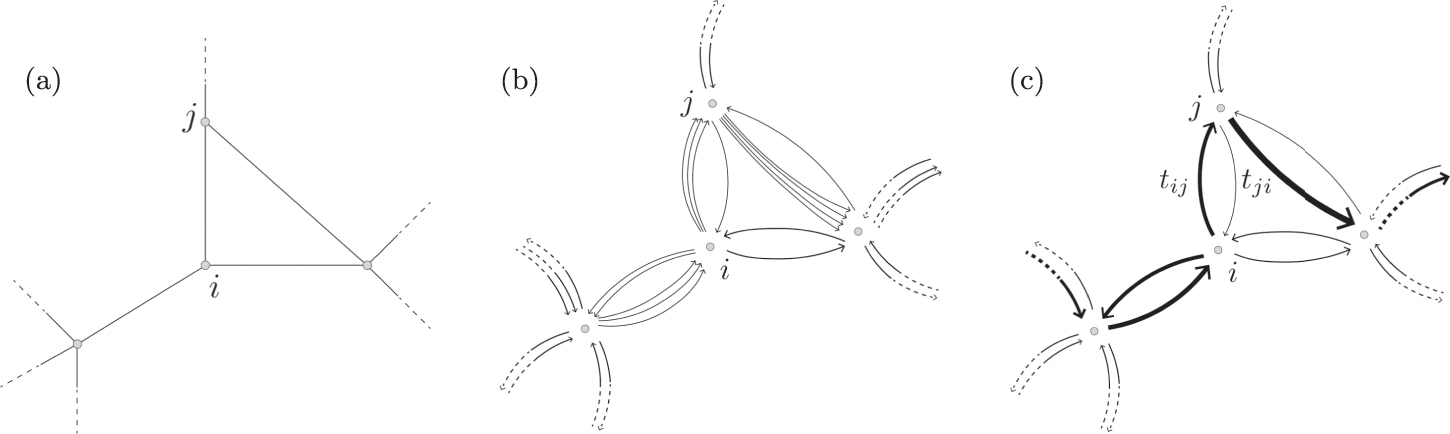
The graph-combinatorial approach is based on the representation of the state space connectivity as a graph G with associated adjacency matrix A—see figure 2(a). This has elements A_ij = 1 if state j can directly be reached from i, and 0 otherwise. In this context, we will refer to states also as nodes or vertices. The transition matrix Π of the Markov chain X, in turn, embeds in its elements the connectivity of the state space as Π_ij = A_ij p_ij with p_ij the jump probability between i and j.

The moment generating function of the probability $\mathbb{P}({L}_{n}^{(2)}=T/n)$ is

$$\begin{equation}{Z}_{N,n}(s)=\sum\limits _{{X}_{1},\dots ,{X}_{n+1}}\mathbb{P}({X}_{1})\prod\limits _{\ell =1}^{n}{{\Pi}}_{{X}_{\ell },{X}_{\ell +1}}\,{\mathrm{e}}^{\sum\limits _{ij}\,{s}_{ij}{\delta }_{{X}_{\ell },\,i}{\delta }_{{X}_{\ell +1},j}},\end{equation} \tag{ 20 }$$

where $\mathbb{P}({X}_{1})$ indicates the probability distribution of our process at initial time n = 1 and $s={({s}_{ij})}_{i,j=1}^{N}$ indicates the set of tilting parameters.

The specific form of the distribution $\mathbb{P}({X}_{1})$ will play a role for finite time behaviour or sub-leading asymptotics, but it will not matter in the large deviation regime—it only amounts to a boundary term—provided that the graph G is strongly connected. For convenience, we choose $\mathbb{P}({X}_{1})={\delta }_{{X}_{1},1}$, viz the starting node is fixed to be node 1.

The core idea of our work is to perform a change of variables: we transform the sum over all states X_ℓ , for ℓ ∈ {1, ..., n + 1}, to a sum over variables t_ij ∈ {0, ..., n}, for nodes i, j ∈ G. The new variable t_ij , as in the previous section 2, is the number of times the Markov chain jumps from state i to state j, in particular t_ij can be different from zero only if there is an edge in G between nodes i and j.

For a matrix T to represent the number of jumps of a chain of states (X₁, X₂, ..., X_n+1) the following constraints must be satisfied: (i) the total number of jumps is equal to the total length of the chain minus one, ∑_ij t_ij = n, (ii) all jumps can be temporally arranged like domino tiles (1, X₂), (X₂, X₃), ..., (X_n , X_n+1) reflecting the fact that if at time ℓ the Markov chain jumps to state i, then at time ℓ + 1 it has to start from state i. Constraints (i) and (ii) do not make the change of variables one to one—there can be many instances of the Markov chain that correspond to the same set of t_ij s. In fact, the variables t_ij do not carry any information regarding the temporal order of the jumps. In other words, given an instance of T we have to count in how many ways we can order the jumps as (1, X₂), (X₂, X₃), ..., (X_n , X_n+1) so that ${\sum }_{\ell =1}^{n}{\delta }_{{X}_{\ell },i}{\delta }_{{X}_{\ell +1},j}={t}_{ij}$ and {X₁, X₂, ..., X_n+1} realises a walk in G: we call this number Θ_T . Hence, we can express Z_N,n as

$$\begin{equation}{Z}_{N,n}(s)=\sum\limits _{{t}_{11}=0}^{n}\dots \sum\limits _{{t}_{ij}=0}^{n}\dots \sum\limits _{{t}_{NN}=0}^{n}{\delta }_{\sum\limits _{ij}{t}_{ij},n}{{\Theta}}_{T}\prod\limits _{i,j}\left({{\Pi}}_{ij}^{{t}_{ij}}\,{\mathrm{e}}^{{s}_{ij}{t}_{ij}}\right).\end{equation} \tag{ 21 }$$

We now face the problem of computing Θ_T . We notice that for many instances of T, this number is simply zero: this is because the aforementioned domino-like constraint (ii) imposes stringent conditions on the form of T. First of all, the set of edges (i, j), for which t_ij > 0, together with the union of all their extremes i and j must form a connected graph. This is because the Markov chain starting from a node i can only hop to neighbours of i according to the connectivity of G. Mathematically, this condition is equivalent to requiring that the dimension of the kernel of the Laplacian L = D_in − T is 1 [42], where D_in is a diagonal matrix with elements ${({D}_{\text{in}})}_{ii}={\sum }_{j}{t}_{ji}$. Second, the number of times a Markov chain jumps towards a state i have to be related to the number of jumps starting from that state i, a phenomenon analogous to the Kirchhoff law in electric circuits that encodes the global balance of the dynamics. We hereby distinguish two possible scenarios in which these conditions on T are satisfied. In the first one, for every state the incoming flux and outgoing flux are equal, that is ∑_j t_ij = ∑_j t_ji : this situation corresponds to a Markov chain starting and ending in the same node, and we will refer to this as the cycle scenario. In the second one, for all but two states the incoming and outgoing fluxes are equal. The two special states are the initial, that we set to 1 choosing $\mathbb{P}({X}_{1})={\delta }_{{X}_{1},1}$, and the final, F, for which one must have ∑_j t_1j = 1 + ∑_j t_j1 and 1 + ∑_j t_Fj = ∑_j t_jF : we will refer to this as the path scenario. This leads to a natural way to express

$$\begin{align}\hfill {{\Theta}}_{T}& ={{\Theta}}_{T}^{\text{path}}\sum\limits _{F\ne 1}\left(\prod\limits _{i\ne 1,F}^{N}{\delta }_{\sum\limits _{j=1}^{N}{t}_{ij},\,\sum\limits _{j=1}^{N}{t}_{ji}}\right){\delta }_{\sum\limits _{j=1}^{N}{t}_{1j}+1,\sum\limits _{j=1}^{N}{t}_{j1}}{\delta }_{\sum\limits _{j=1}^{N}{t}_{Fj},\,\sum\limits _{j=1}^{N}{t}_{jF}+1}\hfill \\ \hfill & \quad +{{\Theta}}_{T}^{\text{cycle}}\prod\limits _{i=1}^{N}{\delta }_{\sum\limits _{j=1}^{N}{t}_{ij},\,\sum\limits _{j=1}^{N}{t}_{ji}}\left(1-{\delta }_{\sum\limits _{j=1}^{N}{t}_{1j},0}\right),\hfill \end{align} \tag{ 22 }$$

where ${{\Theta}}_{T}^{\text{path}}$ $({{\Theta}}_{T}^{\text{cycle}})$ is the number of distinct permutations of the set of t_ij s in the path (cycle) scenario which give a realisation of a walk in G and the deltas enforce Kirchhoff law. The factor $1-{\delta }_{{\sum }_{j=1}^{N}{t}_{1j},0}$ ensures that the cycle will pass at least once from node 1: this condition is required because the starting node is node 1. We will show that it is not necessary to enforce connectedness explicitly because the expressions for ${{\Theta}}_{T}^{\text{path}}$ and ${{\Theta}}_{T}^{\text{cycle}}$ are automatically zero when T is not connected.

We now note that we can interpret the matrix T as the adjacency matrix of a directed multi-graph M_T with t_ij directed links, having unitary weight, between nodes i and node j—see figure 2(b). A directed multi-graph is a collection of nodes and directed links, in which multiple links between two nodes are permitted. We refer to the collection of links between two nodes as a multi-link. As a preliminary step in the computation of ${{\Theta}}_{T}^{\text{path}}$ $({{\Theta}}_{T}^{\text{cycle}})$, we consider a related combinatorial problem, that is counting how many paths there are on M_T that start in 1 and end in F (cycles that start in 1) and pass through every link exactly once. We can interpret this as the number of non-distinct ways we can arrange the jumps like domino tiles that respect the matrix of jumps T. This number overestimates ${{\Theta}}_{T}^{\text{path}}$ (respectively ${{\Theta}}_{T}^{\text{cycle}}$). To see this, we can consider a multi-link in M_T having at least two links l₁ and l₂. Given a path (or cycle) that passes through every link in M_T , we can, for instance, generate another distinct one by swapping the order in which we visit l₁ and l₂. This new path (cycle) will not contribute to ${{\Theta}}_{T}^{\text{path}}$ $({{\Theta}}_{T}^{\text{cycle}})$, as the time-ordered jumps (1, X₂), (X₂, X₃), ..., (X_n , X_n+1) are unaffected by the swap. Nonetheless, this calculation is a useful starting point as we can compute this number using results available in the literature [43], and we will show how to correct this overcounting later on.

So far we have described the key steps that underlie our approach, which are also summarised in the flowchart in figure 1. In the following instead we will provide the details of the calculation. For this reason, some definitions will be useful and we collect them in this paragraph. An Eulerian multi-graph is a multi-graph for which, at every node i, in-degree and out-degree are the same, viz ${k}_{i}^{\mathrm{i}\mathrm{n}}={k}_{i}^{\text{out}}$. Noticing that in M_T we have ${k}_{i}^{\mathrm{i}\mathrm{n}}={\sum }_{j}{t}_{ji}$ and ${k}_{i}^{\text{out}}={\sum }_{j}{t}_{ij}$, it follows from Kirchhoff law that M_T is either an Eulerian multi-graph (for the cycle scenario) or close to an Eulerian multi-graph (for the path scenario), in the sense that only the initial and final nodes do not satisfy k_in = k_out. An Eulerian cycle (path) on a multi-graph M_T , as already mentioned in section 2, is a cycle (path) that passes through every link exactly once. We denote the number of Eulerian cycles (paths) with ec(M_T ) (ep(M_T )). Furthermore, we will indicate by ec(M_T |χ) (ep(M_T |χ)) the number of Eulerian cycles (paths) given some specified condition χ, that in our case will be a combination of the starting node 1, the final node F, the starting edge e₁ and the final edge e_F.

Zoom In Zoom Out Reset image size

In the literature on the topic, a result is known for the number ec(M_T |e₁) of Eulerian cycles of an Eulerian multi-graph M_T with a fixed starting edge. This goes by the name of BEST theorem [43–45] and reads

$$\begin{equation}ec({\mathbf{M}}_{T}\vert {e}_{1})={{\Omega}}_{w}({\mathbf{M}}_{T})\prod\limits _{i=1}^{N}({k}_{i}^{\mathrm{i}\mathrm{n}}-1)!,\end{equation} \tag{ 23 }$$

where Ω_w (M_T ) is the number of arborescences, i.e., spanning trees rooted in a node w such that there exists a unique path from every vertex of M_T to w. We note that Ω_w does not depend on the choice of root w when M_T is an Eulerian multi-graph, so that Ω_w (M_T ) = Ω(M_T ) [44, 46]. Similarly, the rhs of (23) does not show any explicit dependence on the starting edge e₁ because of the inherent symmetry in M_T . An explicit expression for Ω(M_T ) is given by

$$\begin{equation}{\Omega}({\mathbf{M}}_{T})=\mathrm{d}\mathrm{e}\mathrm{t}({L}_{w}),\end{equation} \tag{ 24 }$$

where det is the determinant operator and L_w is a submatrix of the Laplacian of the Eulerian multi-graph M_T obtained by removing (any) wth row and column, a result known in the literature as Tutte's theorem or Matrix tree theorem.

In the following, we first consider the path scenario. In this case, the multi-graph M_T is not Eulerian, but we can make it so simply by adding a link e_F from F to 1. We refer to this modified graph as ${\tilde{\mathbf{M}}}_{T}$. Using BEST theorem we have

$$\begin{equation}ec({\tilde{\mathbf{M}}}_{T}\vert {e}_{1})={\Omega}({\tilde{\mathbf{M}}}_{T})\prod\limits _{i\ne 1}^{N}\left(\sum\limits _{j=1}^{N}{t}_{ji}-1\right)!\left(\sum\limits _{j=1}^{N}{t}_{j\,1}\right),\end{equation} \tag{ 25 }$$

where we use the fact that the in-degree of node 1 is ${\sum }_{j=1}^{N}{t}_{j1}+1$ in ${\tilde{\mathbf{M}}}_{T}$. The number of Eulerian cycles starting from node 1 is related to $ec({\tilde{\mathbf{M}}}_{T}\vert {e}_{1})$ by $ec({\tilde{\mathbf{M}}}_{T}\vert 1)=ec({\tilde{\mathbf{M}}}_{T}\vert {e}_{1})\left({\sum }_{j}\,{t}_{j1}+1\right)$. Furthermore, ep(M_T |1, F) is equal to the number of Eulerian cycles in ${\tilde{\mathbf{M}}}_{T}$ starting in 1 and ending with the link we added to construct it, viz $ec({\tilde{\mathbf{M}}}_{T}\vert 1,{e}_{F})$. This number can be computed by considering an Eulerian cycle in M_T as a collection of loops passing through node 1. The number of these loops is given by the in-degree of node 1, so that we have $ep({\mathbf{M}}_{T}\vert 1,F)=ec({\tilde{\mathbf{M}}}_{T}\vert 1)/({\sum }_{j}{t}_{j1}+1)$. All these considerations put together give

$$\begin{equation}ep({\mathbf{M}}_{T}\vert 1,F)={{\Omega}}_{1}({\mathbf{M}}_{T})\prod\limits _{i\ne 1}^{N}\left(\sum\limits _{j=1}^{N}{t}_{ji}-1\right)!\left(\sum\limits _{j=1}^{N}{t}_{j\,1}\right),\end{equation} \tag{ 26 }$$

where we used ${\Omega}({\tilde{\mathbf{M}}}_{T})=\mathrm{det}({L}_{1})={{\Omega}}_{1}({\mathbf{M}}_{T})$ with L₁ the cofactor of the graph Laplacian L obtained by removing the first row and column. We note that while ${\Omega}({\tilde{\mathbf{M}}}_{T})$ does not depend on the choice of the root since ${\tilde{\mathbf{M}}}_{T}$ is Eulerian, Ω₁(M_T ) does, because M_T is not Eulerian.

We now consider the cycle scenario. In this case, since M_T is already an Eulerian graph, we can readily express ec(M_T , 1) as

$$\begin{equation}ec({\mathbf{M}}_{T}\vert 1)=ec({\mathbf{M}}_{T}\vert {e}_{1})\sum\limits _{j=1}^{N}{t}_{j\,1}={\Omega}({\mathbf{M}}_{T})\prod\limits _{i\ne 1}^{N}\left(\sum\limits _{j=1}^{N}{t}_{ji}-1\right)!\left(\sum\limits _{j=1}^{N}{t}_{j\,1}\right).\end{equation} \tag{ 27 }$$

As previously argued, ep(M_T |1, F) (ec(M_T |1)) overestimates ${{\Theta}}_{T}^{\text{path}}$ $({{\Theta}}_{T}^{\text{cycle}})$. To correct this, one must consider all the links belonging to a given multi-link as totally equivalent. This boils down to considering a weighted graph W_T (see figure 2(c)) in place of the multi-graph M_T . The weighted graph W_T has adjacency matrix T and directed links (e.g., between nodes i and j) obtained by merging all the multi-links (between i and j) in M_T together. In analogy with [45], we define the notion of T-Eulerian cycle (path) as a cycle (path) that passes through every link (i, j) a number t_ij of times. With an abuse of notation, we denote the number of T-Eulerian cycles (paths) by ec(W_T |χ) (ep(W_T |χ)), as it will be clear by the graph we are considering whether we are referring to Eulerian or T-Eulerian cycles (paths). Crucially, in the cycle scenario ${{\Theta}}_{T}^{\text{cycle}}$ is equal to the number of T-Eulerian cycles starting from node 1, i.e., ec(W_T |1) in W_T , whereas in the path scenario ${{\Theta}}_{T}^{\text{path}}$ is equal to the number of T-Eulerian paths from 1 to F, i.e., ep(W_T |1, F) in W_T . The combinatorial factor connecting ep(W_T |1, F) (ec(W_T |1)) to ep(M_T |1, F) (ec(M_T |1)) is simply the number of permutations of links in a multi-link for every multi-link in M_T

$$\begin{equation}\begin{array}{cccc}ep({\mathbf{M}}_{T}\vert 1,F)& =ep({\mathbf{W}}_{T}\vert 1,F)\prod\limits _{i,j=1}^{N}{t}_{ij}!\\ ec({\mathbf{M}}_{T}\vert 1)& =ec({\mathbf{W}}_{T}\vert 1)\prod\limits _{i,j=1}^{N}{t}_{ij}!.\end{array}\end{equation} \tag{ 28 }$$

Zoom In Zoom Out Reset image size

This allows us to write explicit expressions for ${{\Theta}}_{T}^{\text{path}}$ and ${{\Theta}}_{T}^{\text{cycle}}$

$$\begin{equation}{{\Theta}}_{T}^{\text{path}}={{\Theta}}_{T}^{\text{cycle}}=\mathrm{det}({L}_{1})\prod\limits _{i=1}^{N}\frac{\left({\sum }_{j=1}^{N}{t}_{ji}-1\right)!}{{\prod }_{j=1}^{N}{t}_{ij}!}\sum\limits _{k=1}^{N}{t}_{k1},\end{equation} \tag{ 29 }$$

where we recall that L₁ is—in both the cycle and the path scenarios—the submatrix of the graph Laplacian L obtained by removing the first row and column. We remark that, although the expressions for ${{\Theta}}_{T}^{\text{path}}$ and ${{\Theta}}_{T}^{\text{cycle}}$ in (29) are formally the same, the variable T is of different nature in the path and cycle scenario as it satisfies different sets of constraints. With this expression, we can write the moment generating function explicitly as

$$\begin{equation}\begin{aligned}\hfill {Z}_{N,n}(s)& =\sum\limits _{{t}_{11}=0}^{n}\dots \sum\limits _{{t}_{ij}=0}^{n}\dots \sum\limits _{{t}_{NN}=0}^{n}{\delta }_{{\sum }_{ij}\,{t}_{ij},n}\prod\limits _{i,j}\left({{\Pi}}_{ij}^{{t}_{ij}}\,{\mathrm{e}}^{{s}_{ij}{t}_{ij}}\right)\mathrm{det}({L}_{1})\hfill \\ \hfill & \quad \times \sum\limits _{j=1}^{N}{t}_{j1}\prod\limits _{i=1}^{N}\frac{\left({\sum }_{j=1}^{N}{t}_{ji}-1\right)!}{{\prod }_{j=1}^{N}{t}_{ij}!}\left(\sum\limits _{F\ne 1}\left(\prod\limits _{i\ne 1,F}^{N}{\delta }_{\sum\limits _{j=1}^{N}{t}_{ij},\sum\limits _{j=1}^{N}{t}_{ji}}\right)\right.\hfill \\ \hfill & \left.\quad \times {\delta }_{\sum\limits _{j=1}^{N}{t}_{1j}+1,\sum\limits _{j=1}^{N}{t}_{j1}}{\delta }_{\sum\limits _{j=1}^{N}{t}_{Fj},\sum\limits _{j=1}^{N}{t}_{jF}+1}\right.\hfill \\ \hfill & \quad \left.+\left(\prod\limits _{i=1}^{N}{\delta }_{\sum\limits _{j=1}^{N}{t}_{ij},\,\sum\limits _{j=1}^{N}{t}_{ji}}\right)\left(1-{\delta }_{{\sum }_{j}\,{t}_{1j},0}\right)\right).\hfill \end{aligned}\end{equation} \tag{ 30 }$$

We note that the factor det(L₁) kills configurations of T that have the null-space dimension of the Laplacian greater than 1. This ensures that we only consider graphs M_T —equivalently, W_T —that are connected, as it is known in the literature that the dimension of the null-space of the graph Laplacian is the number of connected components of a graph [42]. Remarkably, in equation (30) the contributions for paths and cycles are split, giving an interesting physical perspective. In general, this difference is more pronounced when n is small, in particular when the walker has not explored the full state space. In the limit of large n, contributions relative to paths and cycles are comparable and share the same asymptotics, as we show in the next section.

Compared to the spectral method to compute the moment generating function [17], which requires the computation of all eigenvalues and eigenvectors of an N × N matrix, our formula is computationally favourable when n is small and N is large. If n is large, instead, the spectral method is numerically more efficient.

Expression (30) is valid for every finite n, and can be used to derive the large n limit and, in principle, finite n corrections. In the following, we focus on the large deviation regime, which corresponds to taking n to be much greater than the longest relaxation time of the system τ(N), n ≫ τ(N). In this limit it is useful to rescale time-additive variables with n as in (17), as we can approximate the sums over t₁₁, ..., t_NN with integrals

$$\begin{equation}\frac{1}{{n}^{\vert {E}_{{\mathbf{W}}_{T}}\vert }}\sum\limits _{{t}_{11}}\dots \sum\limits _{{t}_{NN}}\to \prod\limits _{i,j}{\int }_{0}^{1}\phantom{\rule{0ex}{0ex}}\mathrm{d}{\nu }_{ij},\end{equation} \tag{ 31 }$$

where $\vert {E}_{{\mathbf{W}}_{T}}\vert$ is the number of directed edges in the weighted graph W_T and ν_ij s are defined as in (17). In the rhs of (31) and in the following, by ∑_ij and ∏_ij we mean sums and products over (i, j) such that (i, j) is a directed link in W_T . To leading order in n we obtain the following asymptotic expressions

$$\begin{equation}\prod\limits _{i,j}\left({{\Pi}}_{ij}^{{t}_{ij}}\,{\mathrm{e}}^{{s}_{ij}{t}_{ij}}\right)\to {\mathrm{e}}^{n\sum\limits _{i=1}^{N}\sum\limits _{j=1}^{N}\left({s}_{ij}+\mathrm{log}{{\Pi}}_{ij}\right){\nu }_{ij}}\end{equation} \tag{ 32 }$$

$$\begin{align}\hfill & \quad \left(\sum\limits _{j=1}^{N}{t}_{j1}\right)\left(\prod\limits _{i=1}^{N}\frac{\left({\sum }_{j=1}^{N}{t}_{ji}-1\right)!}{{\prod }_{j=1}^{N}{t}_{ij}!}\right)\to {\mathrm{e}}^{n\sum\limits _{i=1}^{N}\sum\limits _{j=1}^{N}{\nu }_{ij}\left(\mathrm{log}\left(\sum\limits _{k=1}^{N}{\nu }_{ik}\right)-\mathrm{log}({\nu }_{ij})\right)}\hfill \end{align} \tag{ 33 }$$

$$\begin{equation}{\delta }_{{\sum }_{ij}{t}_{ij},n}\to {\delta }_{{\sum }_{ij}{\nu }_{ij},1}\end{equation} \tag{ 34 }$$

$$\begin{equation}{n}^{\vert {E}_{{\mathbf{W}}_{T}}\vert }\to {\mathrm{e}}^{\vert {E}_{{\mathbf{W}}_{T}}\vert \mathrm{l}\mathrm{o}\mathrm{g}n}.\end{equation} \tag{ 35 }$$

The Kirchhoff constraints tend to the same form for large n, giving explicitly

$$\begin{align}\hfill & \quad \sum\limits _{F\ne 1}\left(\prod\limits _{i\ne 1,F}{\delta }_{\sum\limits _{j=1}^{N}{t}_{ji},\sum\limits _{j=1}^{N}{t}_{ij}}\right){\delta }_{\sum\limits _{j=1}^{N}{t}_{j1}+1,\sum\limits _{j=1}^{N}{t}_{1j}}{\delta }_{\sum\limits _{j=1}^{N}{t}_{jF},1+\sum\limits _{j=1}^{N}{t}_{Fj}}\hfill \\ \hfill & \to (N-1)\prod\limits _{i=1}^{N}{\delta }_{\sum\limits _{j=1}^{N}{\nu }_{ji},\sum\limits _{j=1}^{N}{\nu }_{ij}}\hfill \end{align} \tag{ 36 }$$

$$\begin{equation}\quad \prod\limits _{i=1}^{N}{\delta }_{\sum\limits _{j=1}^{N}{t}_{ji},\sum\limits _{j=1}^{N}{t}_{ij}}\to \prod\limits _{i=1}^{N}{\delta }_{\sum\limits _{j=1}^{N}{\nu }_{ji},\sum\limits _{j=1}^{N}{\nu }_{ij}}.\end{equation} \tag{ 37 }$$

We also notice that

$$\begin{equation}\mathrm{det}({L}_{1})={n}^{N-1}\,\mathrm{det}\left(\frac{{L}_{1}}{n}\right)={\mathrm{e}}^{(N-1)\mathrm{log}n+\mathrm{Tr}\left[\mathrm{log}\left(\frac{{L}_{1}}{n}\right)\right]}\to {\mathrm{e}}^{(N-1)\mathrm{log}n},\end{equation} \tag{ 38 }$$

where we use the fact that the determinant is multi-linear in the rows and that each element in L₁ is proportional to n by construction, so that $\mathrm{Tr}\left[\mathrm{log}\left(\frac{{L}_{1}}{n}\right)\right]$ is finite for large n. Remarkably det(L₁) becomes sub-leading in the large n limit, while it may be an interesting term to study the finite-time transient behaviour of the Markov chain. Finally, the term ${\delta }_{{\sum }_{j}\,{t}_{1j},0}$ present in the factor $1-{\delta }_{{\sum }_{j}\,{t}_{1j},0}$ becomes negligible for large n.

Putting all together, we obtain to exponential leading order in n

$$\begin{align}{Z}_{N,n}(s)& \approx {\int }_{0}^{1}\dots {\int }_{0}^{1}\phantom{\rule{0ex}{0ex}}\left(\prod\limits _{i,j}\mathrm{d}{\nu }_{ij}\right){\mathrm{e}}^{n[{\sum }_{ij}\;{\nu }_{ij}(\mathrm{l}\mathrm{o}\mathrm{g}({\sum }_{k}{\nu }_{ik})-\mathrm{l}\mathrm{o}\mathrm{g}({\nu }_{ij}))+{\sum }_{ij}\;({s}_{ij}+\mathrm{l}\mathrm{o}\mathrm{g}{{\Pi}}_{ij})\;{\nu }_{ij}]}\\ & \quad \times \left(\prod\limits _{i}{\delta }_{\sum\limits _{j}{\nu }_{ji},\;\sum\limits _{j}{\nu }_{ij}}\right){\delta }_{{\sum }_{ij}{\nu }_{ij},1}.\end{align} \tag{ 39 }$$

We note that the integrand in (39) can be brought to the form ${\mathrm{e}}^{n{\lambda }_{N}[\nu ]}$, with the following definitions:

$$\begin{equation}{\lambda }_{N}[\nu ]={\lambda }_{1}[\nu ]+{\lambda }_{2}[\nu ]+{\lambda }_{3}[\nu ]+{\lambda }_{4}[\nu ]\end{equation} \tag{ 40 }$$

$$\begin{equation}{\lambda }_{1}[\nu ]=\sum\limits _{i=1}^{N}\sum\limits _{j=1}^{N}{\nu }_{ij}\left(\mathrm{log}\left(\sum\limits _{k=1}^{N}{\nu }_{ik}\right)-\mathrm{log}({\nu }_{ij})\right)\end{equation} \tag{ 41 }$$

$$\begin{equation}{\lambda }_{2}[\nu ]=\sum\limits _{i=1}^{N}\sum\limits _{j=1}^{N}\mathrm{log}({{\Pi}}_{ij})\,{\nu }_{ij}\end{equation} \tag{ 42 }$$

$$\begin{equation}{\lambda }_{3}[\nu ]=\sum\limits _{i=1}^{N}\sum\limits _{j=1}^{N}{s}_{ij}\,{\nu }_{ij}\end{equation} \tag{ 43 }$$

$$\begin{equation}{\lambda }_{4}[\nu ]={\epsilon}\left(\sum\limits _{i=1}^{N}\sum\limits _{j=1}^{N}{\nu }_{ij}-1\right)+\sum\limits _{i=1}^{N}{\eta }_{i}\left(\sum\limits _{j=1}^{N}{\nu }_{ij}-\sum\limits _{j=1}^{N}{\nu }_{ji}\right),\end{equation} \tag{ 44 }$$

where and η_i are Lagrange multipliers fixing the respective constraints. In (40) each term has a clear physical interpretation: λ₁, in (41), is the geometric—viz related to the connectivity of the graph G—entropy of a random walk on a graph with nodes and links contributions, akin to the entropy of a free particle; λ₂, in (42), is the entropy due to the dynamics, encoded in the transition matrix; λ₃, in (43), is the tilting potential necessary to drive the system towards a fluctuation of the pair empirical occupation measure; finally, λ₄ in (44), enforces the normalisation and Kirchhoff-law (global balance).

We can calculate the leading order in n of (39) via a saddle-point approximation, arriving at

$$\begin{equation}{Z}_{N,n}(s)\approx {\mathrm{e}}^{n{\lambda }_{N}[{\nu }^{\ast }]},\end{equation} \tag{ 45 }$$

where ν* = argmin_ν,,η   λ_N [ν] and ν* are the minimisers of λ_N [ν] with respect to the set of ν_ij s, η_i s and . From the Euler–Lagrange equations for critical points of (40), we find the following implicit expression for ${\nu }_{ij}^{\ast }$:

$$\begin{equation}{\nu }_{ij}^{\ast }={({{\Pi}}_{s})}_{ij}\left(\frac{{\text{e}}^{-{\eta }_{j}}}{{\mathrm{e}}^{-{\epsilon}}\;{\text{e}}^{-{\eta }_{i}}}\right)\sum\limits _{k=1}^{N}{\nu }_{jk}^{\ast },\end{equation} \tag{ 46 }$$

where the tilted matrix introduced in (19) appears. From (46) we can write self-consistent conditions for and η_i as follows:

$$\begin{equation}\sum\limits _{j}{\left({{\Pi}}_{s}\right)}_{ij}\,{\text{e}}^{-{\eta }_{j}}={\mathrm{e}}^{-{\epsilon}}\,{\text{e}}^{-{\eta }_{i}}\end{equation} \tag{ 47 }$$

$$\begin{equation}\sum\limits _{i}{\left({{\Pi}}_{s}\right)}_{ij}\frac{{\sum }_{k}\,{\nu }_{ik}^{\ast }}{{\text{e}}^{-{\eta }_{i}}}={\mathrm{e}}^{-{\epsilon}}\frac{{\sum }_{k}\,{\nu }_{jk}^{\ast }}{{\text{e}}^{-{\eta }_{j}}},\end{equation} \tag{ 48 }$$

which reveal that e⁻ is an eigenvalue of the tilted matrix Π_s with right eigenvector components ${r}_{i}={\text{e}}^{-{\eta }_{i}}$ and left eigenvector components ${l}_{j}={\sum }_{k}{\nu }_{jk}^{\ast }/{\text{e}}^{-{\eta }_{j}}$. Substituting (47) into (40) we get

$$\begin{equation}{\lambda }_{N}[{\nu }^{\ast }]=-{\epsilon},\end{equation} \tag{ 49 }$$

and, in particular, since λ_N [ν*] is a maximum, e is the dominant eigenvalue of (19). The same conclusion can be reached by noticing that the left and right eigenvector elements in (47) and (48) are all positive, which is true only for the dominant eigenvalue. These arguments provide a direct link with spectral methods. In particular, (49) provides an expression for the logarithm of the dominant eigenvalue of the tilted matrix.

Remarkably, this approach also provides an alternative expression for the so-called driven (or effective) process. This is a modified Markov chain that explains how specific fluctuations are created in time [1, 20, 36, 37]; under certain conditions, it is equivalent to the original Markov chain conditioned to visiting the fluctuation of interest. Useful spectral and variational expressions of the driven process already appeared in the papers just mentioned. Here, we offer another explicit variational representation valid for discrete-time Markov chains. In agreement with [20], the minimisers ${\nu }^{\ast }=\left\{{\nu }_{ij}^{\ast }\right\}$ of the action functional (40) characterise the driven process transition matrix with components

$$\begin{equation}{\tilde{{\Pi}}}_{ij}=\frac{{\nu }_{ij}^{\ast }}{{\sum }_{k=1}^{N}{\nu }_{ik}^{\ast }}.\end{equation} \tag{ 50 }$$

This last expression offers an alternative way to physically study and simulate the appearance of fluctuations and rare events in discrete-time Markov chain models.

Concluding, in (40) we have obtained λ_N , the SCGF associated with the probability distribution of the pair empirical occupation measure in (4). To get the rate functional (2) we only need to Legendre–Fenchel transform the SCGF in (40), i.e.,

$$\begin{align}\underset{s}{\mathrm{s}\mathrm{u}\mathrm{p}}(\sum\limits _{i=1}^{N}\sum\limits _{j=1}^{N}{s}_{ij}{\nu }_{ij}^{\ast }-{\lambda }_{N}[{\nu }^{\ast }])& =\underset{s}{\mathrm{s}\mathrm{u}\mathrm{p}}({\lambda }_{3}[{\nu }^{\ast }]-{\lambda }_{N}[{\nu }^{\ast }])\\ & =-{\lambda }_{1}[{\nu }^{\ast }]-{\lambda }_{2}[{\nu }^{\ast }]-{\lambda }_{4}[{\nu }^{\ast }]=H[{\nu }^{\ast }],\end{align} \tag{ 51 }$$

where in the last step we recognise the pair empirical rate functional (with the necessary constraints—mentioned and understood in (2)–fixed by the Lagrange multipliers in λ₄).

Assuming that one is interested in studying large fluctuations of an observable of the form (1), we remark that the associated SCGF can be obtained simply replacing λ₃[ν] in (43) with

$$\begin{equation}{\lambda }_{3}[\nu ]=s\sum\limits _{i,j=1}^{N}f(i,j){\nu }_{ij},\end{equation} \tag{ 52 }$$

where s is the tilting parameter conjugated to C_n . For instance, in physics applications, it is often of interest to consider the empirical current ${\mathbb{J}}_{n}(i,j)={L}_{n}^{(2)}(i,j)-{L}_{n}^{(2)}(j,i)$, viz the antisymmetric part of the pair-empirical occupation measure in (4), or again the occupation measure itself ${L}_{n}(i)={\sum }_{j=1}^{N}{L}_{n}^{(2)}(i,j)$. The empirical current is an important observable as it allows us to estimate how far a system lies from equilibrium, whereas the occupation measure gives an estimate of the time spent by the system in each state of the state space.

The moment generating function can be computed using spectral methods. We start from (20) (restricted to the case of the observable (54)), i.e.,

$$\begin{equation}{Z}_{N,n}(s)=\sum\limits _{{X}_{1},\dots ,{X}_{n+1}}\mathbb{P}({X}_{1})\prod\limits _{\ell =1}^{n}{{\Pi}}_{{X}_{\ell },{X}_{\ell +1}}\;{\mathrm{e}}^{s{\delta }_{{X}_{\ell },1}{\delta }_{{X}_{\ell +1},2}},\end{equation} \tag{ 55 }$$

which can be cast in the form

$$\begin{equation}{Z}_{N,n}(s)=\langle {\mathbb{P}}_{1}\vert {\left({{\Pi}}_{s}\right)}^{n}\vert 1\rangle ,\end{equation} \tag{ 56 }$$

where $\langle {\mathbb{P}}_{1}\vert =(1,0)$ is the vector of initial probabilities, |1⟩ = (1, 1) and Π_s is the tilted matrix, viz (19) restricted to the case at hand, which reads

$$\begin{equation}{{\Pi}}_{s}=\left(\begin{matrix}\hfill 1-p\hfill & \hfill p\,{\mathrm{e}}^{s}\hfill \\ \hfill q\hfill & \hfill 1-q\hfill \end{matrix}\right).\end{equation} \tag{ 57 }$$

We can use the spectral decomposition of Π_s to get

$$\begin{align}{Z}_{2,n}(s)& =\langle {P}_{0}\vert (\vert {r}^{+}\rangle \langle {l}^{+}\vert {{\Lambda}}_{+}^{n}+\vert {r}^{-}\rangle \langle {l}^{-}\vert {{\Lambda}}_{-}^{n})\vert 1\rangle \\ & ={r}_{1}^{+}{{\Lambda}}_{+}^{n}({l}_{1}^{+}+{l}_{2}^{+})+{r}_{1}^{-}{{\Lambda}}_{-}^{n}({l}_{1}^{-}+{l}_{2}^{-}),\end{align} \tag{ 58 }$$

where Λ_± are the eigenvalues of Π_s and l^±, r^± the corresponding left and right eigenvectors, respectively. We notice that—for the spectral decomposition of Π_s to be valid—left and right eigenvectors have to be bi-orthonormal.

By computing the eigenvalues and eigenvectors of Π_s explicitly, we arrive at

$$\begin{equation}\begin{aligned}\hfill {Z}_{2,n}(s)& =\frac{1}{{2}^{n+1}\sqrt{{(p-q)}^{2}+4pq\,{\mathrm{e}}^{s}}}\hfill \\ \hfill & \quad \times \left\{\left((1-2\,{\mathrm{e}}^{s})p-q\right)\left[{\left(2-p-q-\sqrt{{(p-q)}^{2}+4pq\,{\mathrm{e}}^{s}}\right)}^{n}\right.\right.\hfill \\ \hfill & \left.\left.\quad -{\left(2-p-q+\sqrt{{(p-q)}^{2}+4pq\,{\mathrm{e}}^{s}}\right)}^{n}\right]\right.\hfill \\ \hfill & \left.\quad \times \left[\sqrt{{(p-q)}^{2}+4pq\,{\mathrm{e}}^{s}}{\left(2-p-q-\sqrt{{(p-q)}^{2}+4pq\,{\mathrm{e}}^{s}}\right)}^{n}\right.\right.\hfill \\ \hfill & \left.\left.\quad +{\left(2-p-q+\sqrt{{(p-q)}^{2}+4pq\,{\mathrm{e}}^{s}}\right)}^{n}\right]\right\}.\hfill \end{aligned}\end{equation} \tag{ 59 }$$

The moment generating function can also be computed using (30). Remarkably, this other formulation highlights two different contributions coming from cycles and paths travelled starting from state 1 of the state space. These can explicitly be written as

$$\begin{align}{Z}_{2,n}^{\text{cycles}}(s)& ={(1-p)}^{n}+\sum\limits _{{t}_{11}=0}^{n}\sum\limits _{{t}_{12}=1}^{n}\sum\limits _{{t}_{22}=0}^{n}{\delta }_{{t}_{11}+2{t}_{12}+{t}_{22},n}{(pq\;{\mathrm{e}}^{s})}^{{t}_{12}}{(1-p)}^{{t}_{11}}{(1-q)}^{{t}_{22}}\\ & \quad \times \left(\genfrac{}{}{0pt}{}{{t}_{11}+{t}_{12}}{{t}_{11}}\right)\left(\genfrac{}{}{0pt}{}{{t}_{22}+{t}_{12}-1}{{t}_{22}}\right)\end{align} \tag{ 60 }$$

$$\begin{align}\hfill {Z}_{2,n}^{\text{paths}}(s)& =\sum\limits _{{t}_{11}=0}^{n}\sum\limits _{{t}_{12}=1}^{n}\sum\limits _{{t}_{22}=0}^{n}{\delta }_{{t}_{11}+2{t}_{12}+{t}_{22}-1,n}\frac{{\left(pq\,{\mathrm{e}}^{s}\right)}^{{t}_{12}}}{q}{(1-p)}^{{t}_{11}}{(1-q)}^{{t}_{22}}\hfill \\ \hfill & \times \left(\genfrac{}{}{0pt}{}{{t}_{11}+{t}_{12}-1}{{t}_{11}}\right)\left(\genfrac{}{}{0pt}{}{{t}_{22}+{t}_{12}-1}{{t}_{22}}\right),\qquad \hfill \end{align} \tag{ 61 }$$

where in ${Z}_{2,n}^{\text{cycles}}(s)$ we made explicit the cycle contribution coming from staying for n consecutive steps on state 1, and in ${Z}_{2,n}^{\text{paths}}(s)$ the counting needs to start from t₁₂ = 1 because to have a meaningful path contribution the Markov chain needs to hop at least once from state 1 to state 2. We remark that in this simple model det(L₁) = t₁₂ if t₁₂ ≠ 0 (in such a case the term is absorbed in (60) and (61) by the binomial coefficients), while when t₁₂ = 0 the Laplacian is a 1 × 1 matrix: L₁ is thus an empty matrix, and we take its determinant to be 1 for consistency.

We can find an explicit expression for (60) and (61) analytically. We replace the delta functions appearing by their contour integral representations

$$\begin{equation}{\delta }_{i,j}=\frac{1}{2\pi i}{\oint }_{\vert z\vert =1}{z}^{i-j-1}\;\mathrm{d}z.\end{equation} \tag{ 62 }$$

After making the substitution, we notice that the integrands in (60) and (61) are analytic functions everywhere except in 0. This allows us to deform the integration contour to a circle of radius ≪ 1. The reason for this is to avoid spurious poles in the following steps.

We now let all the sums run up to ∞. This procedure is allowed as higher order terms in the sums do not affect the residue in 0. The infinite sums can be explicitly evaluated and by doing so we get

$$\begin{align}\hfill {Z}_{2,n}^{\text{cycles}}(s)& ={(1-p)}^{n}+\frac{1}{({\mathrm{e}}^{s}pq-pq+q+p-1)}\frac{1}{2\pi \mathrm{i}}\hfill \\ \hfill & \quad \times {\oint }_{\vert z\vert ={\epsilon}}\frac{1}{{z}^{n-1}}\frac{{\mathrm{e}}^{s}pq}{(z(1-p)-1)(z-{z}_{1}^{\ast })(z-{z}_{2}^{\ast })}\hfill \end{align} \tag{ 63 }$$

$$\begin{equation}{Z}_{2,n}^{\text{paths}}(s)=-\frac{1}{({\mathrm{e}}^{s}pq-pq+q+p-1)}\frac{1}{2\pi \mathrm{i}}{\oint }_{\vert z\vert ={\epsilon}}\frac{1}{{z}^{n}}\frac{{\mathrm{e}}^{s}p}{(z-{z}_{1}^{\ast })(z-{z}_{2}^{\ast })},\end{equation} \tag{ 64 }$$

where

$$\begin{equation}\qquad {z}_{1}^{\ast }=\frac{2}{2-p-q-\sqrt{{(p-q)}^{2}+4\,{\mathrm{e}}^{s}pq}}\end{equation} \tag{ 65 }$$

$$\begin{equation}{z}_{2}^{\ast }=\frac{2}{2-p-q+\sqrt{{(p-q)}^{2}+4\;{\mathrm{e}}^{s}pq}}.\end{equation} \tag{ 66 }$$

Notice that ${z}_{1}^{\ast }$ and ${z}_{2}^{\ast }$ are exactly the inverse of the eigenvalues found with spectral methods. We remark that the integrands in (63) and (64) have acquired new singularities, in the form of simple poles at ${z}_{1}^{\ast }$, ${z}_{2}^{\ast }$ and 1/(1 − p): these poles are unphysical, in the sense that their residue should not be considered when computing the contour integrals.

We can express ${Z}_{2,n}^{\text{cycles}}(s)$ and ${Z}_{2,n}^{\text{paths}}(s)$ as

$$\begin{align}{Z}_{2,n}^{\text{cycles}}(s)& ={(1-p)}^{n}+\frac{1}{({\mathrm{e}}^{s}pq-pq+q+p-1)}{\mathrm{R}\mathrm{e}\mathrm{s}}_{z=0}\\ \hfill & \quad \times \left(\frac{1}{{z}^{n-1}}\frac{{\mathrm{e}}^{s}pq}{(z(1-p)-1)(z-{z}_{1}^{\ast })(z-{z}_{2}^{\ast })}\right)\hfill \end{align} \tag{ 67 }$$

$$\begin{equation}{Z}_{2,n}^{\text{paths}}(s)=-\frac{1}{({\mathrm{e}}^{s}pq-pq+q+p-1)}\,{\mathrm{R}\mathrm{e}\mathrm{s}}_{z=0}\left(\frac{1}{{z}^{n}}\frac{{\mathrm{e}}^{s}p}{(z-{z}_{1}^{\ast })(z-{z}_{2}^{\ast })}\right).\end{equation} \tag{ 68 }$$

Computing the residues we find

$$\begin{align}\hfill {Z}_{2,n}^{\text{cycles}}(s)& ={(1-p)}^{n}\hfill \\ & \quad +\frac{({\mathrm{e}}^{s}pq{({z}_{2}^{\ast })}^{-n}({z}_{1}^{\ast }({({z}_{2}^{\ast }/{z}_{1}^{\ast })}^{n}-{({z}_{2}^{\ast }-p{z}_{2}^{\ast })}^{n})+{z}_{2}^{\ast }(-1+{({z}_{2}^{\ast }-p{z}_{2}^{\ast })}^{n}+(-1+p){z}_{1}^{\ast }(-1+{({z}_{2}^{\ast }/{z}_{1}^{\ast })}^{n}))))}{({\mathrm{e}}^{s}pq-pq+p+q-1)((1+(-1+p){z}_{1}^{\ast })({z}_{1}^{\ast }-{z}_{2}^{\ast })(1+(-1+p){z}_{2}^{\ast }))}\end{align} \tag{ 69 }$$

$$\begin{align}\hfill {Z}_{2,n}^{\text{paths}}(s)& =\frac{({\mathrm{e}}^{s}p{({z}_{2}^{\ast })}^{-n}(-1+{({z}_{2}^{\ast }/{z}_{1}^{\ast })}^{n}))}{({\mathrm{e}}^{s}pq-pq+q+p-1)({z}_{1}^{\ast }-{z}_{2}^{\ast })}.\hfill \end{align} \tag{ 70 }$$

By summing these two contributions and replacing ${z}_{1}^{\ast }$ and ${z}_{2}^{\ast }$ from (65) and (66), we obtain exactly (59).

In figure 3 we show the functions ${Z}_{2,n}^{\text{cycles}}$ and ${Z}_{2,n}^{\text{paths}}$ and compare them with the moment generating function previously obtained via spectral methods.

Zoom In Zoom Out Reset image size

Evidently, the moment generating function obtained by summing up cycles and paths contributions completely matches the moment generating function obtained with spectral methods, as the two curves are indistinguishable. An advantage of the graph-combinatorial approach with respect to the spectral calculation is the possibility to split the contributions coming from cycles and paths. As expected for the simple model investigated, cycles contribute less to the moment generating function for s > 0 with respect to paths, and viceversa for s < 0. The reason for this is that in the path scenario the Markov chain has to jump at least once from 1 to 2, contributing to C_n . The larger the n, the less pronounced is this effect. We also show in figure 4 the ratio ${Z}_{2,n}^{\text{cycles}}/{Z}_{2,n}^{\text{paths}}$ for a few fixed values of the tilting parameter s as a function of time n. Noticeably, the ratios become constant for n big enough, supporting the fact that both ${Z}_{2,n}^{\text{cycles}}$ and ${Z}_{2,n}^{\text{paths}}$ share the same asymptotics for large n and differ only by a constant prefactor that is a function of s.

Zoom In Zoom Out Reset image size

We now investigate fluctuations in the large-n limit computing the SCGF λ(s). We compare the spectral and the variational formulae, to highlight the benefits of both approaches.

Using the spectral approach, the logarithm of the dominant eigenvalue is the SCGF (59) and reads

$$\begin{equation}\lambda (s)=\mathrm{log}\,\frac{2-p-q+\sqrt{{(p-q)}^{2}+4pq\,{\mathrm{e}}^{s}}}{2}.\end{equation} \tag{ 71 }$$

We can arrive at the same result by minimising (40). Noticing that Kirchhoff law reduces to ν₁₂ = ν₂₁, the action functional reduces to

$$\begin{align}\lambda [\nu ]& =({\nu }_{11}+{\nu }_{12})\mathrm{l}\mathrm{o}\mathrm{g}({\nu }_{11}+{\nu }_{12})+({\nu }_{12}+{\nu }_{22})\mathrm{l}\mathrm{o}\mathrm{g}({\nu }_{12}+{\nu }_{22})\\\ & \quad -\mathrm{l}\mathrm{o}\mathrm{g}\;{\nu }_{11}-\mathrm{l}\mathrm{o}\mathrm{g}\;{\nu }_{22}+{\nu }_{11}\;\mathrm{l}\mathrm{o}\mathrm{g}(1-p)+{\nu }_{12}(\mathrm{l}\mathrm{o}\mathrm{g}\;p+\mathrm{l}\mathrm{o}\mathrm{g}\;q)\\ & \quad +{\nu }_{22}\;\mathrm{l}\mathrm{o}\mathrm{g}(1-q)+s{\nu }_{12}+{\epsilon}({\nu }_{11}+2{\nu }_{12}+{\nu }_{22}-1).\end{align} \tag{ 72 }$$

The determinant of the system of equations satisfied by the minimum of (73), which is linear in ν, must be 0 to have non-trivial solutions. This condition gives an equation for e⁻ ( is the Lagrange multiplier fixing the normalisation condition) whose solution gives—through (49)—expression (72). This last can be replaced in the form of the minimisers obtained by solving the linear system, which read

$$\begin{equation}{\nu }_{11}^{\ast }=\frac{{(1-q)}^{-1}\,{\mathrm{e}}^{-{\epsilon}}-1}{{(1-q)}^{-1}\,{\mathrm{e}}^{-{\epsilon}}+2({(1-p)}^{-1}\,{\mathrm{e}}^{-{\epsilon}}-1)({(1-q)}^{-1}\,{\mathrm{e}}^{-{\epsilon}}-1)+{(1-p)}^{-1}\,{e}^{-{\epsilon}}-2}\end{equation} \tag{ 73 }$$

$$\begin{equation}{\nu }_{12}^{\ast }=\frac{({(1-p)}^{-1}\,{\mathrm{e}}^{-{\epsilon}}-1)({(1-q)}^{-1}\,{\mathrm{e}}^{-{\epsilon}}-1)}{{(1-q)}^{-1}\,{\mathrm{e}}^{-{\epsilon}}+2({(1-p)}^{-1}\,{\mathrm{e}}^{-{\epsilon}}-1)({(1-q)}^{-1}\,{\mathrm{e}}^{-{\epsilon}}-1)+{(1-p)}^{-1}\,{\mathrm{e}}^{-{\epsilon}}-2}\end{equation} \tag{ 74 }$$

$$\begin{equation}{\nu }_{22}^{\ast }=\frac{{(1-p)}^{-1}\;{\mathrm{e}}^{-{\epsilon}}-1}{{(1-q)}^{-1}\;{\mathrm{e}}^{-{\epsilon}}+2({(1-p)}^{-1}\;{\mathrm{e}}^{-{\epsilon}}-1)({(1-q)}^{-1}\;{\mathrm{e}}^{-{\epsilon}}-1)+{(1-p)}^{-1}\;{\mathrm{e}}^{-{\epsilon}}-2},\end{equation} \tag{ 75 }$$

to get their explicit form as a function of p, q, and the tilting parameter s.

In the top-left and bottom-left panels of figure 5 we plot the minimisers (74)–(76) as a function of the tilting parameter s. For the top-left case, we use p = q = 0.5, while for the bottom case p = 0.5 and q = 0.9. We notice that when p = q, as in the top-left panel, ${\nu }_{11}^{\ast }={\nu }_{22}^{\ast }$ identically. This reflects a permutation symmetry of the system: when p = q, switching states 1 and 2 does not affect the transition matrix. In this case, the Markov chain smoothly transitions between two regimes: for s ≪ 0, the chain spends half of the time in node 1 and half on 2; for s ≫ 0, the chain spends all the time jumping from state 1 to state 2 and back. When p ≠ q, instead, for s < 0 the system smoothly transitions to a localised state, where the Markov chain is mostly located on 1 (resp. 2) if p < q (resp. p > q). Interestingly, we notice that for p < q the maximum of ${\nu }_{22}^{\ast }$ occurs at a finite and negative value of s.

Zoom In Zoom Out Reset image size

In the top-right and bottom-right panels of figure 5 we plot each contribution to the SCGF obtained with our approach alongside their sum. The SCGF is in perfect agreement with the one obtained using spectral methods. Furthermore, our approach allows us to understand the magnitude of each physical term. We split λ₁(s), as defined in (41), into two terms as follows:

$$\begin{equation}{\lambda }_{1,\text{states}}=\sum\limits _{i=1}^{2}\sum\limits _{j=1}^{2}{\nu }_{ij}\,\mathrm{log}\left(\sum\limits _{k=1}^{2}{\nu }_{ik}\right)\end{equation} \tag{ 76 }$$

$$\begin{equation}{\lambda }_{1,\text{links}}=-\sum\limits _{i=1}^{2}\sum\limits _{j=1}^{2}{\nu }_{ij}\;\mathrm{l}\mathrm{o}\mathrm{g}({\nu }_{ij}),\end{equation} \tag{ 77 }$$

and plot them separately. In the top-right panel we used p = q = 0.5, while in the bottom-right panel we used p = 0.5 and q = 0.9. In both cases, when |s| is large we notice that λ_1,states and λ_1,links balance each other, and their sum is close to zero. This is because in both cases, the Markov chain spends most of the time in just a fraction of the available links. For s ≫ 0, the dominant contribution in both cases is due to the tilting term λ₃(s). For s ≪ 0, we notice a striking difference: when p = q, both λ_1,states and λ_1,links tend to a finite value. This is because the chain still visits both node 1 and node 2. Instead, in the case p ≠ q, λ_1,states and λ_1,links tend to 0. This is because of the aforementioned localisation behaviour. In both cases, since the tilting term λ₃(s) becomes negligible, the SCGF λ is well approximated by λ₂, the dynamical entropy.