
Abstract
Anomalous diffusion phenomena are observed in many areas of interest. They manifest themselves in deviations from the laws of Brownian motion (BM), e.g. in the non-linear growth (mostly power-law) in time of the ensemble average mean squared displacement (MSD). When we analyze the real-life data in the context of anomalous diffusion, the primary problem is the proper identification of the type of the anomaly. In this paper, we introduce a new statistic, called empirical anomaly measure (EAM), that can be useful for this purpose. This statistic is the sum of the off-diagonal elements of the sample autocovariance matrix for the increments process. On the other hand, it can be represented as the convolution of the empirical autocovariance function with time lags. The idea of the EAM is intuitive. It measures dependence between the ensemble-averaged MSD of a given process from the ensemble-averaged MSD of the classical BM. Thus, it can be used to measure the distance between the anomalous diffusion process and normal diffusion. In this article, we prove the main probabilistic characteristics of the EAM statistic and construct the formal test for the recognition of the anomaly type. The advantage of the EAM is the fact that it can be applied to any data trajectories without the model specification. The only assumption is the stationarity of the increments process. The complementary summary of the paper constitutes of Monte Carlo simulations illustrating the effectiveness of the proposed test and properties of EAM for selected processes.
Export citation and abstract BibTeX RIS

Original content from this work may be used under the terms of the Creative Commons Attribution 4.0 licence. Any further distribution of this work must maintain attribution to the author(s) and the title of the work, journal citation and DOI.
1. Introduction
Anomalous diffusion phenomena are observed in many areas of interest. They manifest themselves in deviations from the laws of Brownian motion (BM), e.g. in the non-linear growth (mostly power-law) in time of the ensemble average mean squared displacement (MSD), namely ![$E\left[{X}^{2}\left(t\right)\right]\sim {t}^{\alpha }$](https://content.cld.iop.org/journals/1751-8121/54/2/024001/revision3/aabcc84ieqn1.gif) , where α is called the anomalous diffusion exponent. Depending on the α parameter one can distinguish between sub-diffusive (α < 1), normal (α = 1), and super-diffusive (α > 1) behavior. Although the anomalous diffusion is mostly considered in the means of ensemble average MSD, this phenomena influences also the probability density function (PDF) of the corresponding process. The classical diffusion is composed by both linear growth of the second moment of the process as well as its Gaussian distribution. Any deviations from these properties are related to the anomalous diffusion, see for instance [1–4].
, where α is called the anomalous diffusion exponent. Depending on the α parameter one can distinguish between sub-diffusive (α < 1), normal (α = 1), and super-diffusive (α > 1) behavior. Although the anomalous diffusion is mostly considered in the means of ensemble average MSD, this phenomena influences also the probability density function (PDF) of the corresponding process. The classical diffusion is composed by both linear growth of the second moment of the process as well as its Gaussian distribution. Any deviations from these properties are related to the anomalous diffusion, see for instance [1–4].
The classical anomalous diffusion models are fractional Brownian motion (FBM) [5, 6], Lévy stable motion [7] and continuous-time random walk [8, 9]. To the class of anomalous diffusion processes, we include also the subordinated processes (called also time-changed processes) [10–13]. The most popular is the time-changed BM driven by the so-called inverse to the strictly increasing Lévy stable subordinator [14–17] for which the PDF is described by the fractional diffusion equation [8]. The family of anomalous diffusion models contains also the processes with time- or position-dependent diffusion coefficients such as scaled BM [18, 19] or heterogeneous diffusion models [20]. It is worth to mention also the superstatistical process where the diffusion coefficient is a random variable [21] or diffusive diffusivity model, called also Brownian yet non-Gaussian diffusion process, where the diffusion coefficient is described by another process (like the Ornstein–Uhlenbeck one) [22]. In the literature, one can also find the processes with resetting [18, 23] that also belong to the large class of the anomalous diffusion models, see also [24–27] and references therein.
The anomalous diffusion processes have found many practical applications, including physical phenomenon [28, 29], finance [30, 31], ecology [32], hydrology [33], biology [34] as well as meteorology and geophysics [6, 35].
When we analyze the real-life data in the context of anomalous diffusion, the primary problem is the proper identification of the type of anomaly. Through the identification of the type of anomaly, we understand the recognition between sub- or super-diffusive regime. In the statistical and application-oriented literature, one can find various methods used in this analysis. One of the most classical approaches is based on the statistics calculated for real-life data. The known approaches applied in the problem of anomalous diffusion behavior recognition and parametrization are based on simple statistics that exhibit specific behavior for different anomaly types (i.e. for sub- and super-diffusive processes). For instance, the time-averaged MSD is one of the classical statistics used to the anomalous diffusive behavior identification as well as the base for the estimation of the anomalous diffusive exponent [36–42]. The detrended fluctuation analysis (DFA)-based algorithms are popular for the detection of long-range dependence (strongly related to the anomalous diffusion) in nonstationary time series, [43–48]. Moreover, the detrended moving-average (DMA)-based methods were used for the so-called scaling exponent analysis [49–53] and to test FBM identification based on real-life data [54]. It should be mentioned, the literature devoted to the statistical tools for anomalous diffusion processes analysis is very rich, see for instance the papers [55–62].
In the case of second-order processes (i.e. finite-variance) the universal and simplest statistics, that can be applied in the considered problem, is the sample autocovariance function (ACVF). For the zero-mean Gaussian processes the ACVF fully characterizes the distribution of the given model. Moreover, the ACVF exhibits different behavior for processes with different anomaly types thus it is a natural candidate for the analysis of the second-order anomalous diffusion models. The sample ACVF is the classical tool for the detection of the long-range dependence strictly related to the anomalous diffusion behavior [63, 64] as well as for testing the FBM [65]. However, most of the methods mentioned above based on the ACVF, utilize this statistic in one specific time lag. For instance, the test for FBM proposed by the authors in [65] requires selecting the specific time lag and the results are based on the value of the statistic only at this point. This approach seems to be effective however much of the information of the model included in ACVF for all arguments is not used.
In this paper, we take a step forward and propose to use the sample ACVF for all available time points (determined by the available trajectory length). We introduce the new statistic, called the empirical anomaly measure (EAM), which is the sum of the off-diagonal elements of the sample autocovariance matrix for the increments process. On the other hand, the EAM can be represented as the convolution of the empirical ACVF with time lags. The idea of the EAM is intuitive. It measures difference between the ensemble-averaged MSD of a given process from ensemble-averaged MSD of the classical BM. Thus, it can be used to measure the distance between the anomalous and normal diffusion. In this article, we prove the main probabilistic characteristics of the EAM statistic and construct the test for the recognition of the anomaly type. The advantage of the proposed approach is the fact that it can be applied to any real-life data without the model specification. The complementary summary of the paper constitutes of Monte Carlo simulations illustrating the effectiveness of the introduced test and properties of EAM for the exemplary process, namely the FBM.
The paper is organized as follows: in section 2 we introduce the idea of the EAM statistic and prove its main probabilistic properties for the general class of second-order processes. Next, in section 3 we examine the FBM and the behavior of EAM for this process. We indicate the different behavior of the considered statistic for different anomaly types. This section is the starting point for the introduction of the test statistic for the anomalous diffusion behavior recognition. In section 4 we describe the testing procedure and by the Monte Carlo simulations, we check its effectiveness for the FBM. The last section concludes the paper and gives a general overview of future research.
2. Empirical anomaly measure
Let us consider the zero-mean second-order process {X(n)} = {X(n), n = 0, 1, ...}, starting at zero with the ACVF ![$\left\{{\gamma }_{X}\left(i,j\right)=\mathbb{E}\left[X\left(i\right)X\left(j\right)\right],\enspace i,j=0,1,\dots \right\}$](https://content.cld.iop.org/journals/1751-8121/54/2/024001/revision3/aabcc84ieqn2.gif) . Moreover, we consider also the corresponding increments process {Y(n)} = {Y(n), n = 0, 1, ...} defined as
. Moreover, we consider also the corresponding increments process {Y(n)} = {Y(n), n = 0, 1, ...} defined as

with the ACVF ![$\left\{{\gamma }_{Y}\left(i,j\right)=\mathbb{E}\left[Y\left(i\right)Y\left(j\right)\right],\enspace i,j=0,1,\dots \right\}$](https://content.cld.iop.org/journals/1751-8121/54/2/024001/revision3/aabcc84ieqn3.gif) . The crucial quantity reflecting the dynamics of the process {X(n)} is the ensemble average MSD that is defined as follows for any n
. The crucial quantity reflecting the dynamics of the process {X(n)} is the ensemble average MSD that is defined as follows for any n

The MSD measures an average squared displacement of the process over a time period τ. The displacement X(n + τ) − X(n) consists of τ unit-time increments, i.e.

Therefore, one can obtain
which simply shows that the MSD is fully determined by the whole dependence structure of the increments process. Precisely, it is a sum of all elements of covariance matrix {γY (i, j), i, j = n, n + 1, ...n + τ − 1} of the increments process {Y(n)}. The special role in this covariance matrix plays the main diagonal {γY (i, i), i = n, n + 1, ..., n + τ − 1} with the constant entry—variance of unit-time increment. The equation (4) can be rewritten as

In the particular case, when the process {X(n)} has stationary increments, and therefore γY (i, j) = γY (i − j), the equation (5) can be rewritten as

Formulas equations (4)–(6) were well studied in the physical literature in terms of particles diffusion and velocity correlation [66–68]. However in this paper, we concentrate more on statistical properties and applicability potential of quantities in equations (4)–(6). From equation (6) one can conclude that the main diagonal of increments covariance matrix builds inside MSD the linear function of time period τ. When the ACVFs γY (⋅) are summable, the dominated convergence theorem yields [69]

Thus, the ensemble average MSD of {X(n)} decays linearly fast. Once, the ACVFs γY
(⋅) stop being summable (super-diffusion), the ensemble average MSD of {X(n)} can grow faster than linearly and the actual rate of increase of ![$\mathbb{E}\left[{X}^{2}\left(\tau \right)\right]$](https://content.cld.iop.org/journals/1751-8121/54/2/024001/revision3/aabcc84ieqn4.gif) is related to the rate of decay of the ACVF γY
(⋅). When the ACVF is summable (the sub-diffusive case), the ensemble average MSD of {X(n)} grows slower than linear function. The rate of increase of
is related to the rate of decay of the ACVF γY
(⋅). When the ACVF is summable (the sub-diffusive case), the ensemble average MSD of {X(n)} grows slower than linear function. The rate of increase of ![$\mathbb{E}\left[{X}^{2}\left(\tau \right)\right]$](https://content.cld.iop.org/journals/1751-8121/54/2/024001/revision3/aabcc84ieqn5.gif) depends on the parameter which characterizes the asymptotic behavior of the ACVF of the increment process. In the case of the anomalous diffusion models, this parameter is equal to the anomalous diffusion exponent α.
depends on the parameter which characterizes the asymptotic behavior of the ACVF of the increment process. In the case of the anomalous diffusion models, this parameter is equal to the anomalous diffusion exponent α.
The second summand in equation (6)—the sum of all off-diagonal entries of increments covariance matrix—gives the information about the deviation of ![$\mathrm{M}\mathrm{S}\mathrm{D}\enspace \mathbb{E}\left[{X}^{2}\left(\tau \right)\right]$](https://content.cld.iop.org/journals/1751-8121/54/2/024001/revision3/aabcc84ieqn6.gif) from the linear function of time τγY
(0). Thus, the following quantity can be considered as a diffusion anomaly measure (AM) of the process {X(n)}
from the linear function of time τγY
(0). Thus, the following quantity can be considered as a diffusion anomaly measure (AM) of the process {X(n)}

Now, let us assume that we possess a finite trajectory {X(n), n = 1, 2, ..., N} of the process {X(n)} and the corresponding trajectory of the increments {Y(n), n = 1, ..., N − 1}. We assume the process {X(n)} has stationary increments. The natural candidate for the estimator of anomaly measure is the statistic that we call the EAM defined as follows

for any τ = 1, 2, ..., N − 1. In the above equation  is the empirical ACVF of {Y(n), n = 1, ..., N − 1} defined as follows
In the following lemma, we will show that the EAM statistic defined in (9) is the unbiased estimator of the anomaly measure defined in (8).
Lemma 2.1. Let us consider the finite trajectory {X(n), n = 1, 2, ..., N} of the zero-mean second-order process {X(n)} with stationary increments. In that case, the corresponding EAM defined in (9) is the unbiased estimator of the anomaly measure given in (8).
Proof. One can show that for the trajectory of the increments {Y(n), n = 1, ..., N − 1} the following holds
That indicates the EAM ( statistic defined in equation (9)) is the unbiased estimator of the anomaly measure given in equation (8).
□
From lemma 2.1, formula (8) and the fact that γY (0) = E[X(1)2] is constant, one can see that the expected value of EAM is negative and decreasing with respect to τ for the sub-diffusive processes while it is positive and increasing function for the super-diffusive case.
In the following lemma, we prove the formula for the variance of the EAM for the general zero-mean Gaussian process with stationary increments.
Lemma 2.2. Let us consider the finite trajectory {X(n), n = 1, 2, ..., N} of the zero-mean Gaussian process {X(n)} with the stationary increments. The variance of the corresponding EAM defined in equation (9) is given by
where {Y(n), n = 1, ..., N − 1} are increments.
Proof. To calculate the variance of the statistic defined in equation (9), first the second moment is calculated
Let us highlight, the above formula (11) is true for any second-order process, without the assumption of the Gaussianity. Let us note, according to the Isserlis' theorem [70], we have that, if {Z(1), ..., Z(n)} is zero-mean multivariate Gaussian random vector, then the following holds

where  is a set of all the distinct pairings of {1, 2..., n}. Using Isserlis' theorem, we get the following
Finally, we obtain that the variance of the estimator is given by formula (10).□
Lemma 2.2 can be generalized for any vector of random variables (without the assumption of multivariate Gaussian distribution). In the following Lemma, we derive the formula for the variance for EAM for any random vector for that the cumulant-generating function [71] exists.
Lemma 2.3. Let us consider the finite trajectory {X(n), n = 1, 2, ..., N} of the process {X(n)} with the stationary increments. If the cumulant-generating functions [71]

exist, where {1, ..., N − 1}4 is the 4-ary Cartesian power of set {1, ..., N − 1}. Then the variance of the EAM defined in equation (9) is given by
where {Y(n), n = 1, ..., N − 1} is the trajectory of the corresponding increments and  is the joint cumulant [71] of
  (for the definition of
  see the equation (15)) with b being the element from the set p taken from P4—the partition of {1, 2, 3, 4}.
Proof. In the considered case the second moment of the statistic defined in equation (9) is given in equation (11). Here we will use the generalization of Isserlis' theorem [70]—the moment-cumulants formula [72], which states that if for a random vector {Z(1), ..., Z(n)} the cumulant-generating function exists (12), then the following holds

where Pn is a partition of {1, 2, ..., n}. In order to utilize the formula from equation (14), the random variables need to have an (arbitrary but fixed) order. This way we define the bijection from the set of the random variables {(Y(j), Y(j + i), Y(l), Y(l + k))} to the set {1, 2, 3, 4}, hence the partition P4 is well defined. Thus, we introduce a new notation

Then, using the formula (14), we get the following

Therefore, taking into consideration the formula for the expected value of EAM given in lemma 2.1, we conclude that the variance of the estimator is given by equation (13).
□
3. Empirical anomaly measure for fractional Brownian motion
The FBM {XH (t), t ⩾ 0} with Hurst index H ∈ (0, 1) is a continuous and centered Gaussian process that starts at zero (almost surely) with ACVF [5, 73–75]

The parameter D in the above equation is called the diffusion coefficient. For given t ⩾ 0, the random variable  . The FBM has stationary increments and is self-similar. Moreover, it is considered as one of the classical process used to describe the anomalous diffusive phenomena. Indeed, for H < 1/2 it exhibits the sub-diffusive behavior while for H > 1/2—super-diffusive one. Moreover, the FBM with H > 1/2 exhibits also the so-called long-range dependence. For H = 1/2, the FBM reduces to the standard BM. Thus, for FBM the anomalous diffusive exponent is equal to α = 2H.
In this paper, we consider the discrete-time FBM, i.e. the process {XH (n)} = {XH (n), n = 0, 1, ...}. Through {YH (n)} we denote the increment process defined in equation (1). Thus, in the examined case, the following holds

Using lemmas 2.1 and 2.2 we can calculate the expected value and the variance of the EAM statistic for FBM. Namely, we have the following
The variance of EAM for FBM has the following form
In figure 1 we present a comparison of the theoretical and empirical expected value of EAM for FBM. To calculate the empirical expected value we simulated 1000 trajectories of length N = 300 for FBM. In panel (a) we present the comparison for the sub-diffusive case, namely for the FBM with H = 0.2. As one can see, the theoretical and empirical expected values are less than zero for all τs. In this case, the statistic notably decreases with increasing τ. Also, one can observe that theoretical and empirical values coincide. In panel (b) we demonstrate the results for the super-diffusive case, namely for the FBM with H = 0.8. In this case, the statistic increases with growing τ and is always higher than zero. The theoretical and empirical values are almost the same.

Figure 1. The comparison of the theoretical and empirical expected value of EAM for H = 0.2 [panel (a)] and H = 0.8 [panel (b)]. In order to calculate the empirical expected value we simulated 1000 trajectories of length N = 300 for FBM with the corresponding H parameter.
Download figure:
Standard image High-resolution imageIn figure 2 we present the comparison of the theoretical and empirical variance of EAM for FBM in log-log scale. To calculate the empirical variance we simulated 1000 trajectories of length N = 300 of FBM. In the panel (a) we present the results for FBM with H = 0.2 and in panel (b)—with H = 0.8. As one can notice, the theoretical and empirical variances coincide. In both cases, the statistic increases with growing τ, but for the super-diffusive case, the variance takes higher values than for the sub-diffusive process [notice the higher scale in panel (b)].
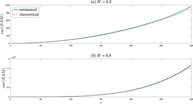
Figure 2. The comparison of the theoretical and empirical variance of EAM for H = 0.2 [panel (a)] and H = 0.8 [panel (b)] (in log–log scale). In order to calculate the empirical variance we simulated 1000 trajectories of length N = 300 for FBM with the corresponding H parameter.
Download figure:
Standard image High-resolution imageIn figure 3 we present the exemplary trajectory of the FBM in the sub-diffusive case (H = 0.2) with D = 1, see the panel (a), and the corresponding EAM statistic for the whole range of τ parameter calculated according to the equation (9), see the panel (b). The length of the trajectory is N = 300. The similar trajectory lengths we observe in real-life data, see for instance [19]. As one can see the values of the statistic for the simulated trajectory are less than zero for all considered τs. Moreover, we have also zoomed the beginning and the end of the plot to see the specific behavior of the EAM statistic for small and large values of the arguments. As one can see, for both considered ranges the statistic takes values smaller than zero and it decreases. However, to demonstrate the overall pattern and the specific behavior of the EAM statistic we have made the M = 1000 Monte Carlo simulations of the FBM with H = 0.2. The length of each simulated trajectory is N = 300. Then, for each trajectory, we calculate the EAM statistic for small (first 20) and large (last 20) values of τ parameter. Finally, on panels (c) and (d) in figure 3 we demonstrate the box-plots of the obtained values. One can see, for all simulated trajectories of FBM with H = 0.2 the value of the statistic is smaller than zero and especially for small values of τ the statistic noticeably decreases for increasing τ. Moreover, the variance of the statistic is smaller than for the large values of τ. For large values of the arguments, the EAM statistic also does not exceed the zero value, however, it is more stabilized (but it still decreases) in contrast to the small range of the τ parameter. The range of the statistic is notably larger than for the small values of the arguments.
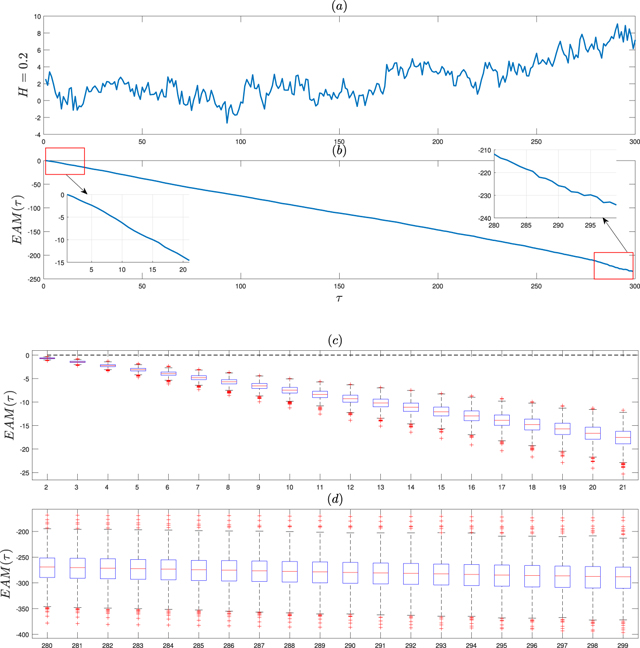
Figure 3. The exemplary trajectory of length N = 300 of FBM with H = 0.2 [panel (a)] and the EAM statistic for this trajectory for the whole range of τ [panel (b)]. The panels (c) and (d) present the box-plots of the EAM statistic values for small [panel (c)] and large [panel (d)] τ parameters. The box-plots are calculated based on M = 1000 Monte Carlo simulations of the FBM with H = 0.2.
Download figure:
Standard image High-resolution imageIn figure 4 we demonstrate the exemplary trajectory of FBM with H = 0.5 and D = 1, i.e. the diffusive case and the corresponding EAM statistic, calculated according to formula (9), see panels (a) and (b), respectively. As one can see, the statistic for the small values of the τ parameters seems to be close to zero, however when we zoomed the plot, one can observe it exceeds a little bit the zero value. When we analyze the large values of the τ parameters, the EAM statistic is smaller than zero and it decreases with increasing τ. Similar as for the sub-diffusive case (i.e. for H = 0.2), we made M = 1000 Monte Carlo simulations of FBM trajectories with H = 0.5 of length N = 300. For each trajectory, we calculate the EAM statistic for all possible τ values (i.e. for τ = 2, 3, ..., 299) and finally in panels (c) and (d) of figure 4 we demonstrate the box-plots of the obtained values for small and large values of the arguments. The medians of the EAM values are close to zero and the variance of the statistic increases along with the τ parameter. This is especially visible for the small values of the τ parameters. However, comparing the sub-diffusive case, we can conclude the statistic is more stabilized.
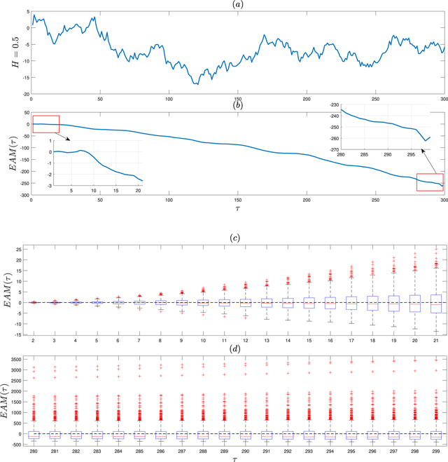
Figure 4. The exemplary trajectory of length N = 300 of FBM with H = 0.5 and D = 1 [panel (a)] and the EAM statistic for this trajectory for the whole range of τ [panel (b)]. The panels (c) and (d) present the box-plots of the EAM statistic values for small [panel (c)] and large [panel (d)] τ parameters. The box-plots are calculated based on M = 1000 Monte Carlo simulations of the FBM with H = 0.5.
Download figure:
Standard image High-resolution imageIn figure 5 we present the exemplary trajectory of length N = 300 for FBM with H = 0.8 (super-diffusive case) and D = 1, see panel (a), and the corresponding EAM statistic, see panel (b). One can clearly see that the statistic increases with respect to the τ parameter and is larger than zero both for small and large values of the arguments. Similar to previous cases, we made M = 1000 Monte Carlo simulations of the sample trajectory of FBM with H = 0.8 of length N = 300 and for each trajectory we calculated the EAM statistic. Finally, we created the box-plots of the obtained values, see panels (c) and (d) of figure 5. The following conclusions can be drawn: for small values of the τ parameters all values of the EAM statistic are higher than zero, this function increases with respect to its arguments and the variance of the statistic also increases. For large values of the τ parameters the median of the EAM statistic is larger than zero, this function is more stabilized than for the small values of the arguments, however the variance of the statistic is larger than for the small values of the τ parameter. One can see the noticeably different behavior of EAM for a super-diffusive case than we have for sub- and diffusive processes.
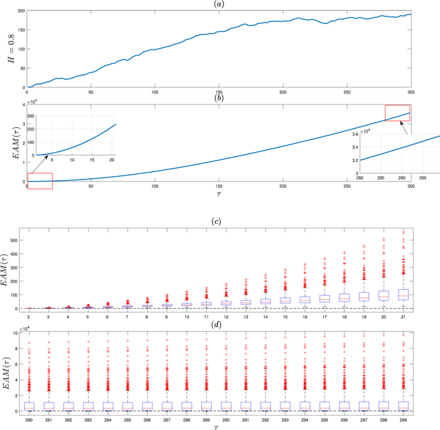
Figure 5. The exemplary trajectory of length N = 300 of FBM with H = 0.8 [panel (a)] and the EAM statistic for this trajectory for the whole range of τ [panel (b)]. The panels (c) and (d) present the box-plots of the EAM statistic values for small [panel (c)] and large [panel (d)] τ parameters. The box-plots are calculated based on M = 1000 Monte Carlo simulations of the FBM with H = 0.8.
Download figure:
Standard image High-resolution imageThe presented simulation results clearly indicate the differences of behavior of the EAM statistic for sub-diffusive, diffusive, and super-diffusive cases. The main differences for the three cases are summarized in the table 1 and became the starting point for proposing a simple test for detecting anomalous behavior in real-life data. The test is precisely described in the next section where we also present its effectiveness for the simulated trajectories of the FBM. Here we present the version for the super-diffusive, behavior testing, but the simple modification of the algorithm allows for testing also the sub-diffusive regime. The main advantage is that the test is model-free and thus it can be used for any processes with a finite second moment.
Table 1. The behavior of the EAM statistic for sub-diffusive, diffusive, and super-diffusive cases.
| Sub-diffusive case | Diffusive case | Super-diffusive case | ||||
|---|---|---|---|---|---|---|
| τ | EAM values | EAM monotonicity | EAM values | EAM monotonicity | EAM values | EAM monotonicity |
| Small | <0 | Decreases | ≈0 | Stabilizes | >0 | Increases |
| Large | <0 | Decreases | ≈0 | Stabilizes | >0 | Increases |
4. Simple test for anomaly detection based on EAM
In this section, we present a simple and intuitive application of the EAM statistic defined in equation (9). As it was mentioned above, the specific behavior of the statistic summarized in table 1 for sub-diffusive, diffusive, and super-diffusive cases can be a starting point for the test for anomalous diffusive behavior detection for real-life data. This test can be applied without the assumption of the specific model behind the data. However, in this section, we demonstrate its effectiveness for simulated trajectories of FBM for different values of the Hurst exponent and three selected trajectory lengths. As one can see in table 1 the EAM statistic can be considered as a detector for the discrimination between sub- and super-diffusive behavior.
Based on our results we can formulate the test with the following hypotheses

The procedure of testing is straightforward. Namely, for the real-life data set x(1), x(2), ..., x(N) of length N first we estimate the EAM according to the formula (9) for selected values of τ parameters. Next, we check the behavior of the statistic along the set of τ values. If the statistic increases and takes values greater than zero we can suspect the super-diffusive regime. In other cases we, reject the H0 hypothesis.
When the number of trajectories from the same experiment is available, then we can calculate the empirical probability that the estimated value of the EAM statistic is greater than zero. We remind, zero is the borderline case discriminating between sub- and super-diffusion. More precisely, if the number of the available trajectories from the same experiment is M, each trajectory is of length N, then for each τ the probability that the EAM is greater than zero can be calculated as follows

where the  is the empirical value of the AM statistic calculated for ith trajectory in point τ (according to equation (9)). If the calculated
  is small (i.e. smaller than the given confidence level) for selected values of the τ parameters one can expect the data do not exhibit super-diffusive behavior. For a large value of
  we do not reject the H0 hypothesis. One can enhance the information obtained for one specific value of τ and analyze the
  for a set of τ parameters.
In our simulation study, we made the following experiment. For each of the analyzed values of N ∈ {50, 100, 300} we simulate M = 1000 trajectories of the FBM for H ∈ {0.01, 0.02, ..., 0.99}. For each H and each τ parameter, we calculate the empirical probability that the EAM is below zero, which is exactly equal to  , where
  is defined as in equation (17). For the test with hypotheses defined as in (16) the empirical probability
  is equal to the power of the test. We remind that the power of the test is the probability that the test rejects the H0 hypothesis when a specific alternative hypothesis H1 is true. The statistical power ranges from 0 to 1, and as statistical power increases, the probability of making a type II error (wrongly failing to reject the null hypothesis) decreases.
In figures 6–8, we present the power of the test for all considered H values for small (first 20 values) and large (last 20 values) τ parameters for three considered values of N. One can see, for small trajectory length N = 50 (see figure 6), the power for H ⩽ 0.3 is equal to one for small and large values of τ parameter, it decreases when H tends to 0.5 however in the neighborhood of 0.5 it is still higher than 0.5. For small τ the test seems to be more effective. For H > 0.6 the power is equal to zero. When we analyze the case with N = 100, see figure 7, the message is more clear. For H < 0.4 the power of the test for small and large values of τ is close to 1 while it is equal to 0 for small τ and H > 0.55. For large values of τ parameter, the test is not so effective as in the case of small values of the arguments of EAM statistic. As we expected, for a larger value of N, namely for N = 300, see figure 8, the power of the test seems to be not effective only in the close neighborhood of H = 0.5 parameter and a small value of τ. For large values of τ the trajectory length has no influence on the power of the test, see panels (b) of figures 6–8.

Figure 6. The power of the test for super-diffusive behavior detection based on the EAM statistic for H ∈ {0.01, 0.02, ..., 0.99} for small [panel (a)] and large [panel (b)] values of τ parameters. In order to calculate the power of the test, we simulated 1000 trajectories of length N = 50 for FBM with the corresponding H parameter.
Download figure:
Standard image High-resolution image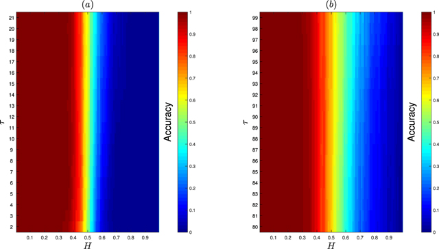
Figure 7. The power of the test for super-diffusive behavior detection based on the EAM statistic for H ∈ {0.01, 0.02, ..., 0.99} for small [panel (a)] and large [panel (b)] values of τ parameters. In order to calculate the power of the test, we simulated 1000 trajectories of length N = 100 for FBM with the corresponding H parameter.
Download figure:
Standard image High-resolution image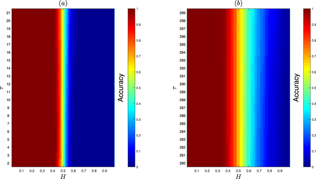
Figure 8. The power of the test for super-diffusive behavior detection based on the EAM statistic for H ∈ {0.01, 0.02, ..., 0.99} for small [panel (a)] and large [panel (b)] values of τ parameters. In order to calculate the power of the test, we simulated 1000 trajectories of length N = 300 for FBM with the corresponding H parameter.
Download figure:
Standard image High-resolution imageIn figures 9–11 in the  and for H = {0.51, 0.52, ..., 0.99}—the
  , where
  is defined in equation (17). The fractions are calculated based on M = 1000 Monte Carlo simulations of the FBM with different values of H parameter. One can see that for the strict sub-diffusive case (H ≪ 0.5) and super-diffusive case (H ≫ 0.5) and small values of τ parameter the calculated empirical probability is equal to zero. However, for the large N, only in the close neighborhood of H = 0.5 the calculated probability is different than 1, however it is still large (∼0.6). The situation is different for large values of τ parameter. Here the calculated probabilities are close to 1 for small values of H parameter. However, when we analyze the case H ≫ 0.5 the calculated values increase but they never meet 1. The presented results clearly indicate the test based on the EAM statistic for anomaly detection is more effective for small values of τ parameter. Obviously, it is also more effective for larger trajectories.
In order to demonstrate the advantages of the proposed approach, we have calculated the computational time of the used testing procedure for the exemplary case. More precisely, for 1000 simulated trajectories of FBM with H = 0.2 with length N we calculated the computational time of the algorithm. Finally, we obtained the mean of the computational times for all trajectories. For the comparison, we have analyzed three trajectory's lengths, namely N = 50, 100 and 300. In table 2 we demonstrate the means of the computational times for two values of τ parameter, namely τ = 2 and τ = N − 1. One can observe the differences of the computational times which follow directly from the definition of the EAM statistic. For larger τ, the number of components used in EAM calculation is larger than for small τ. However, one can see that even for a large value of τ the proposed algorithm is relatively fast.
Table 2. The means of the computational times (in seconds) of testing algorithm based on EAM statistic for H = 0.2 and three values of trajectory lengths N = 50, 100 and 200. To calculate the means we considered 1000 trajectories for each length. The calculations were provided for τ = 2 and τ = N − 1.
| N | τ = 2 | τ = N − 1 |
|---|---|---|
| 50 | 1.417 98 × 10−5 | 1.469 83 × 10−4 |
| 100 | 1.418 99 × 10−5 | 2.921 16 × 10−4 |
| 300 | 1.484 52 × 10−5 | 8.350 19 × 10−4 |
For the implementation of the test and the simulation study, we used MATLAB R2017a. Simulations were performed on Intel(R) Core(TM) i7-7700HQ CPU @ 2.80 GHz.
5. Conclusions and future work
In this paper, we have introduced a new statistic, called the EAM, which is useful in the problem of anomalous diffusion behavior recognition for the second-order processes. Its construction requires the whole information of sample ACVF of the given process (i.e. the ACVF for all arguments) and it is defined as the convolution of the ACVF with appropriate time lags. Thus, the proposed approach utilizes the whole information about the process in contrast to the classical approaches, where the methods are based on the ACVF in a specific time lag. The idea of the EAM is intuitive. It measures the deviation of the ensemble-averaged MSD of the considered process from the ensemble-averaged MSD for the classical diffusion model, namely BM. Thus, the EAM is a natural candidate for the detection of the anomaly type. The proven probabilistic characteristics for the considered statistic indicate this statement. By using the Monte Carlo simulations we have shown that EAM exhibits different behavior for different anomaly types. Thus, we proposed a simple test for the super-diffusive behavior recognition based on real-life data. For the exemplary anomalous diffusion process, namely FBM, we have demonstrated the effectiveness of the proposed approach. The proposed methodology is relatively simple. It utilizes the EAM statistic which is based on the sample ACVF and takes under consideration the fact that the EAM is decreasing with respect to τ and negative for sub-diffusive processes while in the super-diffusive case it increases and takes positive values. Moreover, the EAM-testing method is computationally fast.
Although in this paper we have shown the application of the EAM in the problem of super-diffusive behavior identification, the considered statistic can be also used for testing the sub-diffusive regime (or the general anomalous diffusive one). The simple modification of the described in section 4 procedure allows the recognition of the anomalous diffusive regime of any type. The universality of the proposed approach comes from the specific behavior of the statistic for different anomaly types. The advantage of the introduced methodology is related to the fact it is model-free and can be applied to real-life data without the knowledge of the theoretical process behind the data. However, the simplifying assumption is the stationarity of the increments. This paper can be useful for practitioners who require the simple intuitive methods and algorithms for the real-life data investigation without the preliminary knowledge about the theoretical foundations related to the testing assumptions.
This paper is the preliminary one in the investigation of the EAM statistic in different directions. On one hand, the probabilistic properties (like distribution) of the EAM should be explored for instance in order to introduce a more strict statistical test for anomaly regime recognition. On the other hand, the considered statistic could be also used for the anomalous diffusion parameter estimation without preliminary knowledge about the model. The described testing procedure could be also enhanced by an introduction to the testing schema the intelligent methods, similar as it is used for other statistics useful in the anomalous diffusion behavior analysis known from the literature, see for instance [61, 76–78]. Moreover, the EAM statistic could be also useful in the problem of the transient diffusion recognition. Thus, based on this methodology one can detect the so-called structure breakpoint for the processes with time-varying anomalous diffusion parameter, see e.g. [56, 79].
: Appendix
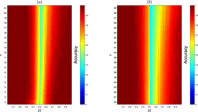
Figure 9. The fraction of values of the EAM statistic that are below zero for H = {0.01, 0.02, ..., 0.5} and above zero for H = {0.51, 0.52, ..., 0.99} for small [panel (a)] and large [panel (b)] values of τ parameters. In order to calculate the empirical probability of anomalous diffusive regime, we considered 1000 trajectories of length N = 50 for each H.
Download figure:
Standard image High-resolution image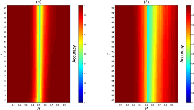
Figure 10. The fraction of values of the EAM statistic that are below zero for H = {0.01, 0.02, ..., 0.5} and above zero for H = {0.51, 0.52, ..., 0.99} for small [panel (a)] and large [panel (b)] values of τ parameters. In order to calculate the empirical probability of anomalous diffusive regime, we considered 1000 trajectories of length N = 100 for each H.
Download figure:
Standard image High-resolution image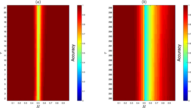
Figure 11. The fraction of values of the EAM statistic that are below zero for H = {0.01, 0.02, ..., 0.5} and above zero for H = {0.51, 0.52, ..., 0.99} for small [panel (a)] and large [panel (b)] values of τ parameters. In order to calculate the empirical probability of anomalous diffusive regime, we considered 1000 trajectories of length N = 300 for each H.
Download figure:
Standard image High-resolution image