
Abstract
Vaccination is commonly used for reducing the spread of infectious diseases; however, we know that not all vaccinations are completely effective. Thus, it is important to study the impacts of vaccine failure on the spreading dynamics of infectious diseases. In this study, we investigate the dynamics of an epidemic model with three types of imperfect vaccinations on complex networks. More specifically, the present model follows a susceptible-infected-susceptible process with a vaccinated compartment that permit leaky, all-or-nothing, and waning vaccines. A threshold value  is first presented to ensure the disease-free equilibrium is asymptotically stable. Next, we derive a necessary and sufficient criterion that assures the presence of a backward (or subcritical) bifurcation when
  . From this criterion, we can observe that the leaky vaccine plays an important role in leading to such a bifurcation, and interestingly, we also find that this condition is independent of the network structure. The disease is also demonstrated to persist whenever
  . Numerical simulations are conducted to validate the theoretical results. Our results show that imperfect vaccination can cause a backward bifurcation, which usually has serious consequences for disease control. Thus, appropriate infection control policies need to be further developed.
Export citation and abstract BibTeX RIS
1. Introduction
In recent times, we have been facing the threat of some infectious diseases such as influenza, HIV/AIDS, dengue, tuberculosis, Zika virus disease, Ebola virus disease, and the recent and rapidly emerging outbreak disease—coronavirus disease 2019 (COVID-19). These infectious diseases usually have a severe impact on human life and the economic system. Therefore, it is urgent to formulate a good epidemic prevention strategy. To prevent and control an infectious disease, we must understand the transmission dynamics of the disease, and try to predict the future evolution of the disease. Mathematical modeling is a powerful tool for analyzing the spread of infectious diseases and this approach has been extensively studied over a period of time [3, 24]. Among the various types of epidemic models, in this study, we are interested in the compartmental models. In a compartmental model, the population is assigned to different compartments according to epidemiological states (e.g., susceptible, infected, exposed, etc), and in a compartment, individuals have the same epidemiological state. Usually, we can formulate a system of differential equations to investigate how the compartments change over time.
Vaccination is recognized as an effective means of disease control and prevention. Therefore, vaccination should play an important role in the transmission dynamics of an infectious disease. There are several compartmental epidemic models that include such a factor to investigate the role of this control strategy [1, 2, 4, 5, 9, 10, 22, 27, 31, 32, 35, 37]. Although vaccination is a useful tool for reducing or eradicating the incidence of an infection, it is well known that not all vaccinations are completely effective. Therefore, it is important to study the effect of imperfect vaccinations on the transmission dynamics of infectious diseases. In general, there are three different types of imperfect vaccinations that are commonly considered in the literature. We use the terminology in [12]: (i) leaky vaccine is used to describe a vaccine that only reduces the probability of infection upon exposure; however, it does not eliminate it; (ii) all-or-nothing vaccine describes a vaccine that has no effect on some individuals but confers complete protection in others; (iii) waning vaccine is the one for which the protection conferred wanes over time. Different epidemic models including all three aforementioned imperfect vaccinations were investigated in [1, 2, 9, 22, 31]. A model that incorporates a nonlinear incidence rate and leaky vaccine was studied in [4]. The epidemic models including all-or-nothing and waning vaccines with a nonlinear incidence rate and a saturated treatment were considered in [5, 10] respectively. A model that incorporates the waning vaccine and general nonlinear incidence was analyzed in [37]. Epidemic models with imperfect vaccination under the impact of opinion dynamics were investigated in [29, 30]. A model that includes the element of vaccine failure and three types of infection awareness and immunization awareness was studied in [15].
Thus far, existing studies have mainly been based on the assumption that individuals in the population are homogeneously mixed. However, it is commonly accepted that contacts among individuals in a population are heterogeneous, and can have vital effects on the transmission of infectious diseases. To describe the effect of contact heterogeneity, the concept of complex networks is included in epidemic modeling. Because of the seminal study by Pastor-Satorras and Vespignani [28], several network-based epidemic models have been proposed and studied [6, 8, 14, 16, 18–20, 25, 33]. It should be noted that there have been relatively fewer studies on network epidemic models with imperfect vaccinations. In [7], two epidemic models incorporating variable population size, degree-related vaccination rate, and quarantine were introduced. Global stability and the conditions for the existence of multiple endemic equilibria were investigated. In [21], the authors studied an epidemic model with imperfect vaccination on scale-free networks. Their model included two degree-related transmission rates and a degree-related vaccination rate. Two threshold parameters were derived, and the existence conditions of multiple endemic equilibria were discussed. Furthermore, the effects of different immunization schemes and an optimal control strategy of vaccination were also presented. Generally, the results of network epidemic models with imperfect vaccinations are still rare. To gain more insight into the effects of imperfect vaccinations on the transmission of infectious diseases, in this study, we investigate a network-based epidemic model with three types of the aforementioned imperfect vaccinations. We first obtain a threshold value  that determines the stability of the disease-free equilibrium. Subsequently, we consider the existence of the endemic equilibrium by a bifurcation analysis. Furthermore, we study the persistence of the disease. Numerical simulations are conducted to validate our theoretical findings. The novelty and contributions of this work are as follows: (i) we not only performed the stability analysis of the disease-free equilibrium, but also studied the bifurcation behavior of the endemic equilibria; (ii) we obtained a necessary and sufficient condition that ensures the occurrence of a backward bifurcation and this condition is independent of network structure; (iii) from our analysis, we observed that the leaky vaccine plays the most important role in the dynamics of epidemic spreading. The leaky vaccine can not only cause the backward bifurcation, but also result in the largest region of backward bifurcation in comparison with the other two imperfect vaccines.
The remainder of this paper is organized as follows. In section 2, we describe the proposed model, and study the stability of the disease-free equilibrium. In section 3, we derive a condition that determines the direction of bifurcating the endemic equilibrium. In section 4, we study the persistence of the disease. In section 5, numerical experiments are detailed to illustrate the theoretical results. Finally, the conclusions are presented in section 6.
2. Model formulation and the disease-free equilibrium
In this section, we present the network-based epidemic model with imperfect vaccinations inspired by the study by Magpantay et al [22]. We assume a population of individuals whose connections to one another form a network. Specifically, in this network, each individual is represented by a node, and the connections among the individuals are formed by edges. The degree of a node is the number of edges between this node and other ones. We classify all the nodes of this network into n groups, such that nodes in the same group have the same degree. This indicates that each node in the kth group has a degree k for k = 1, 2, ..., n, where n is the maximal degree of the network. Furthermore, in each group, we divide the nodes into three categories: susceptible, infected, and vaccinated. Let Sk (t), Ik (t), and Vk (t) represent the densities of susceptible, infected, and vaccinated nodes with node degree k at time t, respectively. The network-based epidemic model is governed by the following system of ordinary differential equations:
where the descriptions of all the parameters are given in table 1. In this model, we assume that the model population has equal birth and natural death rates of μ. The term (1 − (1 − ɛA
)p)μ describes that a fraction p of the newborns are assumed to be vaccinated, and of this fraction, a proportion ɛA
exhibit vaccine failure (i.e., all-or-nothing vaccine). The term βkSk
(t)Θ(t) represents the incidence, and the factor Θ(t) is the probability of a given edge to be connected to an infected node. Specifically, the probability that an edge is connected to a node with degree h is proportional to hP(h), where P(h) > 0 represents the probability of a node with degree h, and hence,  . Thus, the probability that a randomly chosen edge is connected to an infected node is given by
where  denotes the average degree of the network. The parameter ɛL
is introduced to model the phenomenon that vaccination may reduce the probability of infection upon exposure; however, it does not completely eliminate susceptibility to infection (i.e., leaky vaccine). In this study, we also assume the waning rate of vaccinated individuals by α = μɛW
/(1 − ɛW
) (cf [22]) such that the parameter
denotes the average degree of the network. The parameter ɛL
is introduced to model the phenomenon that vaccination may reduce the probability of infection upon exposure; however, it does not completely eliminate susceptibility to infection (i.e., leaky vaccine). In this study, we also assume the waning rate of vaccinated individuals by α = μɛW
/(1 − ɛW
) (cf [22]) such that the parameter

The parameter γ stands for the recovery rate of infected individuals. Let Nk (t) = Sk (t) + Ik (t) + Vk (t) for all k = 1, 2, ..., n. It follows from system (1) that Nk '(t) = μ − μNk (t). Thus, we assume that the initial values satisfy the normalization condition, namely, Nk (0) = Sk (0) + Ik (0) + Vk (0) = 1 for all k, then, we have Nk (t) = 1 for all t ⩾ 0 and k = 1, 2, ..., n. Therefore, we consider the dynamics of the solutions of system (1) in the following biologically meaningful region:

and the initial values are given in Ω. It is easy to verify that Ω is a positively invariant set for system (1), that is, every trajectory of (1) starting in Ω remains in Ω for all t ⩾ 0.
Table 1. Description of parameters.
| Parameters | Description |
|---|---|
| μ ⩾ 0 | Birth and death rates |
| β > 0 | Transmission rate |
| p ∈ [0, 1] | Infant vaccination probability |
| γ > 0 | Recovery rate |
| ɛA ∈ [0, 1) | Probability of not getting protected after vaccination |
| ɛL ∈ [0, 1) | Reduction in the probability of getting infected after vaccination |
| ɛW ∈ [0, 1) | Probability that protection wanes in the case given that one does not get infected first |
| α ⩾ 0 | Waning rate of vaccine-derived immunity |
To find the equilibrium solutions for system (1), we can observe that there always exists a disease-free equilibrium  with
with

Next, we investigate the stability of the disease-free equilibrium  . We first establish the local stability of
  , and subsequently, we consider the global stability of
  . The proofs of the stability results of
  are given in appendix
Theorem 2.1. Define the threshold value
where  . The disease-free equilibrium
  is locally asymptotically stable if
  , and it is unstable if
  .
.
Remark 1. Given that α = μɛW /(1 − ɛW ), one can derive that
where  is the threshold value in the absence of vaccination (p = 0). It can be seen that incorporating an effective vaccine can reduce the threshold value. Therefore, vaccination can prevent the outbreak of diseases.
From remark 1, we can observe that  . The following result shows that
  is globally asymptotically stable when
  .
.


3. Bifurcation analysis
From theorem 2.2, we only obtain the global stability of  when
when  instead of
  . This indicates that the condition
  is not sufficient to eliminate the disease. Therefore, it is important to discuss whether the disease can persist even if
  . In this section, we characterize whether there exists a backward (or subcritical) bifurcation at
  . When such a bifurcation occurs, there exists a range of the threshold value
  (i.e.,
  ) that we refer to as the region of metastability. In this region, there are at least two endemic equilibria and typically, at least one of which is stable. This implies that
  is not globally stable when
  , and the disease can persist even if
  . There are some mechanisms that have been identified to induce such a bifurcation. More precisely, epidemic models can exhibit backward bifurcation owing to mechanisms such as nonlinear treatment rates [10, 17, 19], vaccine failure [1, 2, 4, 9, 31], and host disease-induced mortality [11]. Besides, a model that considers a coupling of an epidemic spreading and an opinion dynamics has been shown to be able to undergo such a bifurcation [30].
Here, we study the bifurcation phenomenon at  . More specifically, we will derive a condition that determines the direction of the bifurcation at
  . Therefore, let us consider the endemic equilibria of system (1). At an endemic equilibrium, we have Sk
, Ik
, Vk
> 0 for all k = 1, 2, ..., n. Furthermore, it should satisfy the following equations:
. Therefore, let us consider the endemic equilibria of system (1). At an endemic equilibrium, we have Sk
, Ik
, Vk
> 0 for all k = 1, 2, ..., n. Furthermore, it should satisfy the following equations:
It can be deduced from the third equation of system (3) that

Combining Sk + Ik + Vk = 1 with the first equation of system (3), we can derive

Substituting the relations (4) and (5) into the second equation of system (3), we can obtain

where Δ1(k, Θ) = ɛL βkΘ + α + μ and Δ2(k, Θ) = βkΘ + α + μ. Substituting relation (6) into the expression of Θ, the following equation can be derived:
Because we are looking for the endemic equilibria, we have Ik > 0 for all k. This implies that Θ > 0. Therefore, the endemic equilibria should obey the following equation of Θ from equation (7):
Once we get Θ from equation (8), Sk
, Ik
, and Vk
can be determined according to the relations (4)–(6). Consequently, the endemic equilibria can be found. We will study the relationship between  and Θ. Therefore, we try to express equation (8) in terms of
  and Θ. From the definition of
  , we set

Therefore, equation (8) becomes
Equation (9) can be used to define an endemic equilibrium curve in the first quadrant of the  -plane. If we treat Θ as a function of
  , the direction of the bifurcation is determined by the slope of the curve at
  . This indicates that if the derivative is negative at the critical value
  , backward bifurcation occurs, and if the derivative at
  is positive, forward bifurcation takes place (figure 1). Therefore, we can obtain a necessary and sufficient criterion that decides the direction of the bifurcation by computing the derivative
  at
at  . To obtain this condition, we differentiate equation (9) implicitly with respect to Rv
, and this leads to the following:
. To obtain this condition, we differentiate equation (9) implicitly with respect to Rv
, and this leads to the following:

where
and
If  and Θ = 0, then
and

Consequently, equation (10) becomes
This implies that
This leads to the following equality:
It should be noted that the left-hand side of equation (11) is positive. Therefore, we can conclude that the sign of  at
at  is the same as the sign of

Consequently, the following necessary and sufficient condition for backward bifurcation can be made:

Figure 1. Schematic bifurcation diagrams. (Left) Forward or supercritical bifurcation (positive slope at  ). (Right) Backward or subcritical bifurcation (negative slope at
  ).
).
Download figure:
Standard image High-resolution imageTheorem 3.1. System (1) has backward bifurcation at  if and only if

Remark 2. From theorem 3.1, we have some observations.
- (a)If p = 0 or ɛL = 0, then condition (12) fails. Therefore, only forward bifurcation occurs at
 . This indicates that if there is no vaccine (i.e., p = 0), then there is only forward bifurcation in our model. However, when a vaccine is present and the protection of the vaccine is not 100% effective, we realize that leaky vaccine plays a vital role, leading to a backward bifurcation.
 - (b)The bifurcation condition (12) is independent of the network structure for our model.
- (c)The bifurcation condition (12) is a necessary and sufficient condition while the conditions derived in [7, 21] are sufficient conditions. This is because we determine the slope of the endemic equilibrium curve at, and in [7, 21], the authors find the conditions to determine the number of endemic equilibria.


4. Persistence of disease
In this section, we study the persistence of the disease by using theorem 4.6 in [34]. It should be noted that the persistence of the disease has the same significance as the global stability of the endemic equilibrium in an epidemiological sense. We briefly sketch the idea of the proof. Define two subsets of Ω, namely,
and

The first step is to show that the set  is a covering of the union of
  , where
  and
and  are the solution and the omega limit set of the solution of system (1) with initial value
  , respectively. The second step is to claim that
  is a weak repeller for X1, i.e.,

Here  denotes the distance between
  and
and  . Owing to theorem 4.6 in [34], the conclusion of persistence can be made. The detailed proof is given in appendix
Theorem 4.1. If  , then there exists an η > 0, which is independent of the initial condition satisfying I(0) > 0, such that
where  .
.
5. Numerical examples
In this section, we present some numerical simulations to illustrate our theoretical results. In the first example, we considered the stability of the disease-free equilibrium  .
.
Example 5.1. In this example, we choose scale-free networks which satisfy a power-law degree distribution, namely, P(k) = η1
k−2.5 for k = 1, 2, ..., 100. The constant η1 is chosen to make  . Therefore, we can get ⟨k⟩ = 1.7995 and ⟨k2⟩ = 13.8643. The parameters of system (1) are selected as β = 0.004, p = 0.85, μ = 0.015, γ = 0.05, ɛL
= 0.2, and ɛA
= ɛW
= 0. Therefore,
. Therefore, we can get ⟨k⟩ = 1.7995 and ⟨k2⟩ = 13.8643. The parameters of system (1) are selected as β = 0.004, p = 0.85, μ = 0.015, γ = 0.05, ɛL
= 0.2, and ɛA
= ɛW
= 0. Therefore,  and
and  can be established. It can be realized from theorem 2.2 that the disease-free equilibrium
  is globally asymptotically stable. We use 30 different initial values to plot the trajectories of Sk
(t), Ik
(t), and Vk
(t) for k = 30, 60, 90. As we can see in figure 2, all the trajectories approach to
is globally asymptotically stable. We use 30 different initial values to plot the trajectories of Sk
(t), Ik
(t), and Vk
(t) for k = 30, 60, 90. As we can see in figure 2, all the trajectories approach to  . This could support that the disease-free equilibrium
  is globally stable.
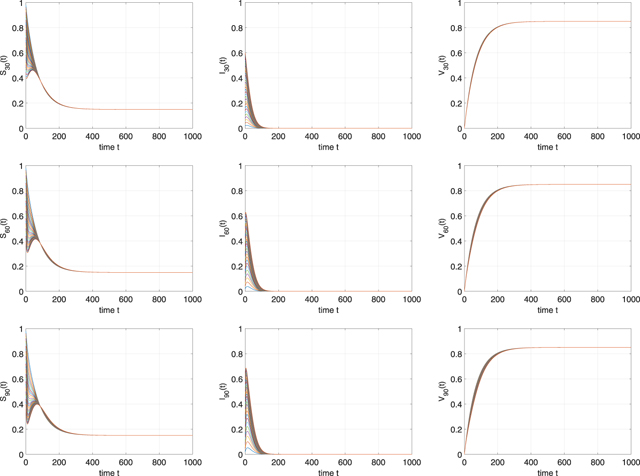
Figure 2. Time evolutions of Sk (t), Ik (t), and Vk (t) for k = 30, 60, 90 in example 5.1. The 30 different initial values are selected as Sk (0) = 1 − 0.02i, Ik (0) = 0.02i, and Vk (0) = 0 for i = 1, 2, ..., 30.
Download figure:
Standard image High-resolution imageExample 5.2. In this example, we consider bifurcation. The following parameters are fixed: β = 0.001, μ = 0.015, and γ = 0.05. In figure 3, we plot phase diagrams with different values of ɛA and ɛW in the parameter domain (ɛL , p) to illustrate condition (12). In the red region, it means that condition (12) is satisfied, and hence, backward bifurcation occurs. On the contrary, forward bifurcation takes place when the parameters are in the blue region. Now, we focus on the left panel of figure 3. If we put p = 0.85 and ɛL = 0.2, then we can verify that

This indicates that condition (12) is met. It can, therefore, be deduced from theorem 3.1 that backward bifurcation occurs at  . However, if we change the value of ɛL
from 0.2 to 0.05, then
. However, if we change the value of ɛL
from 0.2 to 0.05, then

Therefore, forward bifurcation occurs at  . Because condition (12) is independent of the network structure, we will consider four different types of networks to demonstrate this result. The first one is the scale-free network that we have chosen in example 5.1; the second one is the network with an exponential degree of distribution, namely, P(k) = η2 e−k/5 for k = 1, 2, ..., 100; the third one is the Poisson network with degree distribution P(k) = η3 e−1515k
/k! for k = 1, 2, ..., 100; the final one is a scientific collaboration network [26] whose degree of distribution is P(k) = η4
k−1.3 e−k/10.7 for k = 1, 2, ..., 100. The constants ηi
(i = 2, 3, 4) are selected to keep each degree of distribution satisfying
. Because condition (12) is independent of the network structure, we will consider four different types of networks to demonstrate this result. The first one is the scale-free network that we have chosen in example 5.1; the second one is the network with an exponential degree of distribution, namely, P(k) = η2 e−k/5 for k = 1, 2, ..., 100; the third one is the Poisson network with degree distribution P(k) = η3 e−1515k
/k! for k = 1, 2, ..., 100; the final one is a scientific collaboration network [26] whose degree of distribution is P(k) = η4
k−1.3 e−k/10.7 for k = 1, 2, ..., 100. The constants ηi
(i = 2, 3, 4) are selected to keep each degree of distribution satisfying  . The bifurcation diagrams for these networks are given in figures 4–7. The numerical results confirm our theoretical analysis.
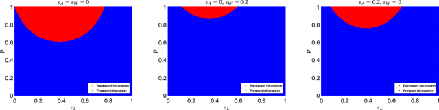
Figure 3. Illustration of condition (12) in the parameter domain (ɛL , p). The fixed model parameters are β = 0.001, μ = 0.015, and γ = 0.05. We also select (left) ɛA = ɛW = 0; (middle) ɛA = 0, ɛW = 0.2; (right) ɛA = 0.2, ɛW = 0. The red region indicates that backward or subcritical bifurcation occurs, and the blue region indicates that forward or supercritical bifurcation takes place.
Download figure:
Standard image High-resolution image
Figure 4. Bifurcation diagrams in the  -plane for scale-free networks. The model parameters are β = 0.001, p = 0.85, μ = 0.015, γ = 0.05, and ɛA
= ɛW
= 0. In the left subfigure, we choose ɛL
= 0.05 and forward bifurcation takes place at
-plane for scale-free networks. The model parameters are β = 0.001, p = 0.85, μ = 0.015, γ = 0.05, and ɛA
= ɛW
= 0. In the left subfigure, we choose ɛL
= 0.05 and forward bifurcation takes place at  . In the right subfigure, we set ɛL
= 0.2. Therefore, backward bifurcation occurs at
. In the right subfigure, we set ɛL
= 0.2. Therefore, backward bifurcation occurs at  .
.
Download figure:
Standard image High-resolution image
Figure 5. Bifurcation diagram in the  -plane for networks with exponential degree of distribution.
Download figure:
Standard image High-resolution image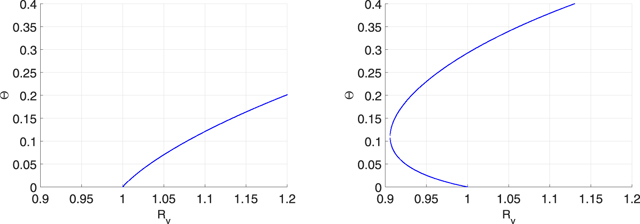
Figure 6. Bifurcation diagrams in the  -plane for the Poisson networks.
Download figure:
Standard image High-resolution image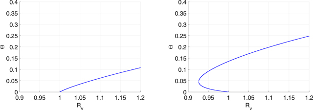
Figure 7. Bifurcation diagrams in the  -plane for a scientific collaboration networks.
Download figure:
Standard image High-resolution imageExample 5.3. In this example, let us focus on the scale-free networks with the degree of distribution described in example 5.1. The parameters are chosen as β = 0.0025, p = 0.85, μ = 0.015, γ = 0.05, ɛL
= 0.2, and ɛA
= ɛW
= 0. Therefore, we have  and
and  . In addition, as we have verified in example 5.2, the condition (12) is satisfied. Therefore, backward bifurcation occurs at
  . Given that
  , it can be observed in the right subfigure of figure 4 that there exist two positive values of Θ, and each of them determines an endemic equilibrium respectively. That is, under the aforementioned parameters, there are two endemic equilibria and one of them is stable. To confirm this observation, 30 different initial values are used to show the time evolutions of Sk
(t), Ik
(t), and Vk
(t) for k = 30, 60, 90. A bistable phenomenon can be observed in figure 8.
, it can be observed in the right subfigure of figure 4 that there exist two positive values of Θ, and each of them determines an endemic equilibrium respectively. That is, under the aforementioned parameters, there are two endemic equilibria and one of them is stable. To confirm this observation, 30 different initial values are used to show the time evolutions of Sk
(t), Ik
(t), and Vk
(t) for k = 30, 60, 90. A bistable phenomenon can be observed in figure 8.

Figure 8. Time evolutions of Sk (t), Ik (t), and Vk (t) for k = 30, 60, 90 in example 5.3. The 30 different initial values are given by Sk (0) = 1 − 0.000 001i, Ik (0) = 0.000 001i, and Vk (0) = 0 for i = 1, 2, ..., 30.
Download figure:
Standard image High-resolution imageExample 5.4. This example is aimed at studying the effects of imperfect vaccines on the backward bifurcation behavior. We fix the parameters β = 0.01, μ = 0.015, γ = 0.2, p = 0.85, and ɛL = 0.2. We will consider the following four cases: (i) ɛA = ɛW = 0; (ii) ɛA = 0.2 and ɛW = 0; (iii) ɛW = 0.2 and ɛA = 0; (iv) ɛA = ɛW = 0.2. The bifurcation diagrams for the different types of network structures are depicted in figure 9, where the bifurcation curves corresponding to case (i)–(iv) are blue, red, black, and magenta respectively. We can observe that the region of metastability depends on the presence of the type of imperfect vaccine. More specifically, the region of backward bifurcation is the largest for case (i), and it is smallest for case (iv). Therefore, it seems that we need the strongest condition to eliminate the disease if there is only a leaky vaccine. However, in the presence of all the three imperfect vaccines, the weakest condition is needed.

Figure 9. Bifurcation diagrams corresponding to the four cases considered in example 5.4 for different network structures.
Download figure:
Standard image High-resolution imageExample 5.5. In the final example, we will conduct simulations to illustrate the persistence of the result. We will still use the scale-free networks with the degree of distribution described in example 5.1. The model parameters are selected as β = 0.03, p = 0.85, μ = 0.015, γ = 0.05 with the 3-tuple (ɛL
, ɛA
, ɛW
) varying. We use 30 different initial values to depict the trajectories of I(t) with different settings of the 3-tuple (ɛL
, ɛA
, ɛW
) in figure 10. As be observed from each panel of figure 9, the threshold value is  . Therefore, the persistence of the disease can be assured from theorem 4.1. In fact, we can see that all the trajectories approach to a positive constant. This indicates that there exists a stable endemic equilibrium when
  .
.
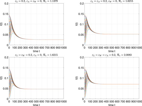
Figure 10. Time evolutions of I(t) in example 5.5. The 30 different initial values are selected as Sk (0) = 1 − 0.005i, Ik (0) = 0.005i, and Vk (0) = 0 for i = 1, 2, ..., 30.
Download figure:
Standard image High-resolution image6. Conclusions
In this study, we investigated the dynamics of a network-based epidemic model with imperfect vaccinations. We considered three types of imperfect vaccinations, namely, leaky, all-or-nothing, and waning vaccines. We proved that there exists a threshold value  that determines the stability of the disease-free equilibrium
  . More specifically, we proved that if
  , then
  is locally asymptotically stable. Furthermore, because of the presence of imperfect vaccinations, we derived a necessary and sufficient condition that ensures the occurrence of a backward (or subcritical) bifurcation at
  . From our result, we found that a leaky vaccine plays a vital role in leading to a backward bifurcation at
  . When such a bifurcation occurs,
  does not confirm the global stability of
  . This means that the condition
  is insufficient to eradicate the disease. When
  , we showed that the disease can persist. Several numerical experiments were performed to validate the theoretical results. We conclude that when a backward bifurcation occurs, we require a stronger condition to eliminate the diseases. In comparison with the three types of imperfect vaccinations, the leaky vaccine must be paid special attention as it explicitly affects the backward bifurcation phenomena, which are challenging from the perspective of disease control. Therefore, it is important to study how to control the spreading dynamics when such a bifurcation has been detected. Furthermore, in this work, we only considered a simple epidemic model on static networks. However, it is known that the real contact networks are time-varying. Hence, it is also necessary to study the spreading dynamics on real contact networks. Besides, we know that disease spread is a fundamentally spatiotemporal phenomenon. Thus, studying the effects of space-time heterogeneities on the spreading dynamics of infectious diseases is also an important and interesting issue. We defer these research topics for future investigation.
Acknowledgments
The authors would like to thank the anonymous referees for their valuable comments and suggestions that improved the presentation of this paper. This work was partially supported by the Ministry of Science and Technology of Taiwan under the Grant MOST 108-2115-M-017-002.
Appendix A.: Stability of the disease-free equilibrium

In this appendix, we give the detailed proofs of the stability results in section 2. The following lemma is used to facilitate the stability analysis.
Lemma A.1. ([36]) For a real n × n matrix A = (aij ) where aij = δij σi + pi qj (pi , qj ⩾ 0, i, j = 1, 2, ..., n) and δij denotes the Kronecker symbol. Then,

Specifically, if σk = σ for all k, then

Proof of theorem 2.1. To determine the local stability of  by linearization, we rearrange the equations in system (1) as the following system:

where  and
and  with yk
(t) = Sk
(t), yn+k
(t) = Ik
(t), y2n+k
(t) = Vk
(t), and
with yk
(t) = Sk
(t), yn+k
(t) = Ik
(t), y2n+k
(t) = Vk
(t), and
Then, we can obtain the Jacobian matrix of system (A.2) at 

where A1 = diag{−μ, −μ, ..., −μ} and A3 = diag{−(α + μ), −(α + μ), ..., −(α + μ)} are two n × n diagonal matrices; O is the n × n zero matrix; A2 is an n × n matrix whose (i, j)-entry is given by
It can be observed that matrix A1 has a negative eigenvalue −μ with multiplicity n, and matrix A3 has a negative eigenvalue −(α + μ) with multiplicity n. Therefore, the other n eigenvalues are determined by the matrix A2. We define the (i, j)-entries of matrix A2 − λI as
Denote

From equation (A.1), the following characteristic polynomial can be made:

By solving the characteristic equation det(A2 − λI) = 0, we can obtain a negative characteristic root λ = −(γ + d) that has multiplicity n − 1. Consequently, the stability of the disease-free equilibrium  completely depends on the sign of the root of
This implies that
Accordingly, if  , then all the eigenvalues of
  are negative. Therefore,
  is asymptotically stable. Conversely, if
  , then
  is unstable because of the existence of a positive eigenvalue. This completes the proof. □
Proof of theorem 2.2. It suffices to show that  is globally attractive, and by combining the local stability result (theorem 2.1), the global stability of
  can be achieved. To this end, first, we claim that Ik
(t) → 0 when t → ∞ for all k. According to the second equation of system (1), we can obtain the derivative of Θ(t):
can be achieved. To this end, first, we claim that Ik
(t) → 0 when t → ∞ for all k. According to the second equation of system (1), we can obtain the derivative of Θ(t):
Given that ɛL ∈ [0, 1) and Ω is a positive invariant set, we can derive that
Because  , we can obtain Θ(t) → 0 as t → ∞. This implies that Ik
(t) → 0 can be considered as t → ∞ for all k. Therefore, for any δ > 0, there exists Tδ
> 0 such that 0 ⩽ Ik
(t) ⩽ δ for t > Tδ
. Next, we claim Vk
(t) → V0 as t → ∞ for all k. It follows from the third equation of system (1) that
, we can obtain Θ(t) → 0 as t → ∞. This implies that Ik
(t) → 0 can be considered as t → ∞ for all k. Therefore, for any δ > 0, there exists Tδ
> 0 such that 0 ⩽ Ik
(t) ⩽ δ for t > Tδ
. Next, we claim Vk
(t) → V0 as t → ∞ for all k. It follows from the third equation of system (1) that

This implies that
In contrast, because 0 ⩽ Ik (t) ⩽ δ for t > Tδ , we have
Considering δ → 0, we can obtain
Therefore, Vk
(t) → V0 when t → ∞ for all k. In fact, Sk
(t) = 1 − Ik
(t) − Vk
(t) leads to Sk
(t) → S0 when t → ∞ for all k. Consequently,  is globally attractive whenever
  , and the proof is completed. □
Appendix B.: Proof of theorem 4.1
and

First, we claim that X1 is a positive invariant with respect to system (1). If (Sk (0), Ik (0), Vk (0)) ∈ X1, then I(0) > 0 and
Therefore, I(t) ⩾ I(0) exp(−(γ + μ)t) is considered for t > 0, making X1 a positive invariant. Furthermore, there is a compact set B in which all the solutions of system (1) initiated in X1 will enter and remain forever. The compactness condition (C4.2) of theorem 4.6 in [34] is easily verified for set B.
Let  be the solution of system (1) with the initial condition
  , and
, and  is the ω-limit set of the solution of system (1) with an initial value of
  . Denote

Restricting system (1) on  gives
gives
Clearly, the disease-free equilibrium  of system (1) is the only equilibrium of system (B.1) in M∂. One can easily claim that
  is globally asymptotically stable in M∂ because (B.1) is a linear system. Therefore,
  . Moreover,
  is a covering of Y. This is isolated and acyclic. Finally, the proof will be completed if we show that
  is a weak repeller for X1, i.e.,

Therefore, we need to verify that  , where
Supposing this is not true, then there exists a solution within the initial condition  such that

Given that  , we can choose a small
  > 0 such that
Considering > 0, there exists T > 0 such that for t > T, and we have

Consider the function  . The derivative of L along solution (Sk
(t), Ik
(t), Vk
(t)) for t > T is given by
. The derivative of L along solution (Sk
(t), Ik
(t), Vk
(t)) for t > T is given by
Because ζ > 1, we can conclude that L(t) → ∞ can be considered as t → ∞. This contradicts the boundedness of L(t). Therefore,  . The proof is completed. □
Appendix C.: Sensitivity and uncertainty analyses
In this appendix, we conduct parameters-related sensitivity and uncertainty analyses on  and on the bifurcation condition (12) since the dynamical behaviors of system (1) are based on these two quantities. We will use Latin hypercube sampling-based method to quantify uncertainty and sensitivity of
  and the left-hand side of condition (12) as a function of 7 parameters (β, γ, μ, p, ɛL
, ɛA
, ɛW
) and a function of 6 parameters (γ, μ, p, ɛL
, ɛA
, ɛW
), respectively. The Latin hypercube sampling is a type of Monte Carlo sampling [13] as it densely stratifies the input parameters. The partial rank correlation coefficient (PRCC) is used as the sensitivity index to measure the impact of the parameters on the output variables, that is,
and the left-hand side of condition (12) as a function of 7 parameters (β, γ, μ, p, ɛL
, ɛA
, ɛW
) and a function of 6 parameters (γ, μ, p, ɛL
, ɛA
, ɛW
), respectively. The Latin hypercube sampling is a type of Monte Carlo sampling [13] as it densely stratifies the input parameters. The partial rank correlation coefficient (PRCC) is used as the sensitivity index to measure the impact of the parameters on the output variables, that is,  and the left-hand side of condition (12). More specifically, the PRCC measures the strength between the input parameters and outputs of the model (i.e.,
  and condition (12)) using correlation through the sampling done by the Latin hypercube sampling method [23]. Because we have no a priori data, a uniform distribution is assigned to each parameter [23]. After using the Latin hypercube sampling method, 2000 samples are taken and the histograms of the input parameter values are drawn in figure 11. Corresponding to the above mentioned distributions for input parameters, the resulting distributions for
  and for the left-hand side of condition (12) are made in figure 12. The distribution of
  is on the left panel of figure 12. In this figure, the probability of
  is about 0.328. The distribution for the left-hand side of condition (12) is on the right panel of figure 12. In this figure, the probability of negative values of condition (12) is about 0.045. The PRCC sensitivity results are carried out for
  and for condition (12), respectively. The bar charts are given in figure 13. PRCC suggests that the parameters β and μ have the highest and the lowest influence on
  , respectively. The parameters ɛW
and ɛL
have the highest and the lowest influence on the bifurcation condition (12), respectively.
, respectively. The parameters ɛW
and ɛL
have the highest and the lowest influence on the bifurcation condition (12), respectively.
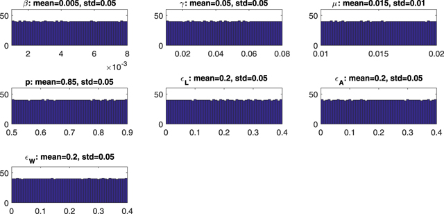
Figure 11. Model parameter distributions from uncertainty analysis.
Download figure:
Standard image High-resolution image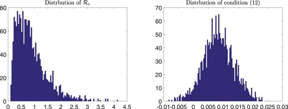
Figure 12. Estimated distributions of  and of the left-hand side of condition (12) based on uncertainty analysis.
Download figure:
Standard image High-resolution image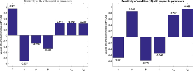
Figure 13. Sensitivity indexes of  (left) and of the left-hand side of condition (12) (right) with respect to their corresponding parameters.
Download figure:
Standard image High-resolution image