
Abstract
We solve the time evolution of a nonlinear optomechanical Hamiltonian with arbitrary time-dependent mechanical displacement, mechanical single-mode squeezing and a time-dependent optomechanical coupling up to the solution of two second-order differential equations. The solution is based on identifying a minimal and finite Lie algebra that generates the time-evolution of the system. This reduces the problem to considering a finite set of coupled ordinary differential equations of real functions. To demonstrate the applicability of our method, we compute the degree of non-Gaussianity of the time-evolved state of the system by means of a measure based on the relative entropy of the non-Gaussian state and its closest Gaussian reference state. We find that the addition of a constant mechanical squeezing term to the standard optomechanical Hamiltonian generally decreases the overall non-Gaussian character of the state. For sinusoidally modulated squeezing, the two second-order differential equations mentioned above take the form of the Mathieu equation. We derive perturbative solutions for a small squeezing amplitude at parametric resonance and show that they correspond to the rotating-wave approximation at times larger than the scale set by the mechanical frequency. We find that the non-Gaussianity of the state increases with both time and the squeezing parameter in this specific regime.
Export citation and abstract BibTeX RIS

Original content from this work may be used under the terms of the Creative Commons Attribution 3.0 licence. Any further distribution of this work must maintain attribution to the author(s) and the title of the work, journal citation and DOI.
1. Introduction
The mathematical understanding of optomechanical systems operating in the nonlinear quantum regime is a major topic of current interest. While most experiments effectively undergo linear dynamics, governed by quadratic Hamiltonians that emerge following a 'linearisation' procedure [1–3], many experiments now operate in the fully nonlinear regime [4–6] where this procedure fails. It is therefore highly desirable to provide a complete and analytic characterisation of the fully nonlinear system dynamics. Analytic solutions have previously been found for a constant light–matter coupling [7, 8] and, more recently, the time-dependent case was solved [9].
The inherently nonlinear interaction between the optical field and the mechanical element in an optomechanical system allows for the generation of non-Gaussian states. Starting from a broad class of initial states, including coherent states, the vacuum, and thermal states, this is only possible in the nonlinear regime; in contrast, quadratic Hamiltonians take input Gaussian states to output Gaussian states. As such, investigating the non-Gaussianity of optomechanical states can only be performed once the time-evolution in the nonlinear regime has been solved, which is the primary aim of this work. Interestingly, a number of non-classical and non-Gaussian states have been found to constitute an important resource for sensing. Schrödinger cat states [7, 8], compass states [10, 11] and hypercube states [12]—which are all non-Gaussian and highly non-classical states—have all been found to have applications for sensing. More generally, the detection and generation of non-Gaussianity in optomechanical systems has been extensively studied in theoretical proposals [13–15] as well as in experiments [4, 5, 16]. Beyond optomechanics, the presence of a nonlinear element is also key to a number of quantum information tasks, such as obtaining a universal gate set for quantum computing [17, 18], teleportation [19], distillation of entanglement [20, 21], error correction [22], and non-Gaussianity has been explored as the basis of an operational resource theory [23–25].
Optomechanical systems offer a natural nonlinear coupling which, if strong enough, may lead to substantial non-Gaussianity in the evolved state. It is therefore essential to better understand the dynamics of such systems, with special emphasis on the interplay between nonlinearities and other Hamiltonian terms in this dynamics. An important question to be answered is thus how do the different aspects of an optomechanical system affect the non-Gaussianity of the state at a given time? A preliminary study of non-Gaussianity in standard optomechanical systems provided the first tools to approach this question [9], however, optomechanical systems can exhibit additional, potentially more interesting, effects. An important non-classical effect that can be included into optomechanical systems is squeezing of the optical or mechanical modes. The addition of squeezing has been found to be beneficial for sensing since it increases the sensitivity in a specific field quadrature. For example, it has been shown that squeezed light injected into LIGO can be used to enhance the detection of gravitational waves [26]. Similarly, mechanical squeezing can aid the amplification and measurement of weak mechanical signals [27].
In this work, we study the non-Gaussianity of a quantum system of two bosonic modes characterised by an optomechanical Hamiltonian with the standard cubic light–matter interaction term, and with the addition of a mechanical displacement term and a mechanical squeezing term. We extend a recently developed solution of the time evolution operator induced by a plain optomechanical Hamiltonian [9] to include the additional terms of interest here. Interestingly, for time-dependent squeezing modulated at resonance, we find that the dynamics are governed by the well-studied Mathieu equation. We subsequently derive perturbaive solutions and show that these coincide with the physically intuitive rotating-wave approximation (RWA) for large times. The decoupling methods used in this work have a long tradition in quantum theory [28–30] and were recently applied to problems such as the one at hand [9, 31, 32]. We use the resulting analytic solutions to compute the amount of non-Gaussianity of the state using a measure of relative entropy [33, 34] for both a constant and a time-dependent mechanical squeezing parameter.
Our results indicate that the non-Gaussian character of an initially coherent state decreases in general with an increasing squeezing parameter. However, when the squeezing is applied periodically at twice the mechanical resonance, the non-Gaussianity increases approximately linearly with time and the amplitude of the squeezing. The competition between the amount of squeezing and the strength of the nonlinear term is difficult to compute explicitly; instead, we provide asymptotic expressions in terms of upper and lower bounds to the non-Gaussianity in different regimes. A conclusive answer requires further investigation, potentially providing a concise expression where such competition can be easily understood.
The paper is structured as follows. In section 2, we introduce the nonlinear Hamiltonian with mechanical squeezing. This is followed by section 3 where we provide a short introduction to the methods used to solve the dynamics. The full derivation can be found in appendix B. Following this, we review the measure of non-Gaussianity and derive expressions for an asymptotic expression and a reduced measure in section 4. In section 5, we then specialise to two specific cases and compute the amount of non-Guassianity for constant squeezing (section 5.2), and for modulated squeezing (section 5.3). Finally, we conclude with a discussion in section 6 and some final remarks in section 7.
2. Dynamics
In this section we present the optomechanical Hamiltonian of interest to this work and explain the origin of the various terms. An extensive introduction to optomechanics can be found in the literature [1].
2.1. Hamiltonian
In this work we consider the two-mode Hamiltonian

where  is the free Hamiltonian, while
  and
and  are the frequencies of the cavity mode and the mechanical resonator respectively.
The Hamiltonian (1) describes the dynamics of a number of different systems. For example,  appears in optomechanical systems as a standard coupling term due to radiation pressure obtained for Fabry–Pérot cavities, where one end of the cavity is a mirror that can move freely [35]. Such coupling appears also within systems with a central translucent membrane in a rigid optical cavity [36], levitated nanodiamonds [37] or optomechanical crystals [38, 39]. A depiction of a levitated nanosphere interacting with cavity modes can be found in figure 1.
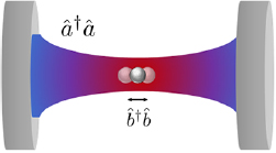
Figure 1. A levitated nanosphere in a cavity. The optical field is described by annihilation and creation operators  and
and  , while the mechanics—in this case the mechanical motion of the nanosphere—is described by annihilation and creation operators
  and
and  . The system evolves under the optomechanical Hamiltonian (2).
Download figure:
Standard image High-resolution imageThe Hamiltonian (1) reduces to the standard optomechanical Hamiltonian when  9. The term weighted by the coupling
  corresponds to an externally imposed displacement of the mechanical part, which can be induced by a piezoelectric element connected to its support or by an external acceleration, such as that caused by the gravitational force acting on the mechanical element [40, 41]. The term governed by
  can be thought of as a modulation of the trap frequency and leads to squeezing of the mechanics, which can be externally imposed employing another strong optical field or an electrostatic force [42].
2.2. Dimensionless dynamics
To understand which dimensionless parameters are relevant to the dynamics of the system, we start by introducing dimensionless quantities and rescaling the Hamiltonian. Such a rescaling also serves to simplify the notation and any graphical representation of the system dynamics. We achieve this by dividing the functions in the Hamiltonian by the mechanical frequency  . The action corresponds to switching from the laboratory time t to
  , where
  is the new, dimensionless time. The optical frequency becomes
  . In addition, the couplings in the Hamiltonian become
  ,
,  and
and  . We also rescale the Hamiltonian by
  , meaning that
  becomes

which is the Hamiltonian that we will be working with.
3. Solving the dynamics
Our aim is to provide the techniques to be used to understand the interplay of mechanical squeezing and non-Gaussianity in an optomechanical system, for which an analytic expression for the state evolution [9] is central. In this section we introduce the tools needed to solve the dynamics generated by (2). See appendix A for a more in-depth introduction to the underlying concepts, and appendix B for the full calculations.
3.1. Continuous variables and covariance-matrix formalism
When solving the dynamics, we employ methods from the continuous variable formalism [3, 43]. Specifically, the methods are used to solve the time-evolution of the quadratic part of the system, and to describe its action on the nonlinear light–matter interaction term. We briefly review the continuous variable formalism here.
In recent years, thanks to progress in the mathematical framework provided by the covariance matrix formalism [3, 43], it has become clear that Gaussian states constitute an extremely valuable toolkit to investigate quantum information processing in quantum setups, and in relativistic ones as well [44]. The main advantage is that the covariance matrix formalism provides a powerful set of mathematical tools to treat Gaussian states of bosonic fields that undergo linear transformations of the creation and annihilation operators fully analytically [43]. Ultimately, Gaussian states are the paramount resource for continuous variables quantum information processing and computation [17] and have become a standard feature in most quantum optics laboratories. However, it should also be pointed out that these methods can be used to describe the evolution of operators in the Heisenberg picture, even when the states considered are not Gaussian.
In quantum mechanics, the initial state  of a system of N bosonic modes with operators
  evolves to a final state
  through the standard Schrödinger equation
  , where
  implements the transformation of interest, such as time evolution. If the state
  is Gaussian and the Hamiltonian
  is quadratic in the operators, it is convenient to introduce the vector
  , where
  denotes the transpose of the vector. Similarly, the vector of first moments
  and the covariance matrix
  are defined by
  , where
  stands for anticommutator and all expectation values of an operator
  are defined by
  .
.
In this language, the canonical commutation relations read ![$ \newcommand{\re}{{\rm Re}} \renewcommand{\dag}{\dagger}[\hat{X}_n,\hat{X}_m^{{\dagger}}]={\rm i}\,\Omega_{nm}$](https://content.cld.iop.org/journals/1751-8121/53/7/075304/revision2/aab64d5ieqn037.gif) , where the
, where the  matrix
  is known as the symplectic form [43]. We then notice that, while arbitrary states of bosonic modes are, in general, characterised by infinite real parameters, a Gaussian state is uniquely determined by its first and second moments, dn and
  respectively [43]. Furthermore, unitary transformations quadratic in the annihilation and creation operators, such as Bogoliubov transformations [45], preserve the Gaussian character of a Gaussian state and can always be represented by a
  symplectic matrix
  that preserves the symplectic form, i.e.
  10. In a similar manner, the symplectic matrix
  that encodes the evolution of a state is generated by the Hamiltonian matrix
  , which is defined by
  . The symplectic matrix becomes
 ![$\boldsymbol{S} = \mathrm{exp} \left[ \boldsymbol{\Omega} \boldsymbol{H}\right]$](https://content.cld.iop.org/journals/1751-8121/53/7/075304/revision2/aab64d5ieqn049.gif) .
.
The Schrödinger equation can be translated in this language to the simple equation  for the second moments, and
  for the first moments, which shifts the problem of usually untreatable operator algebra to simple
  matrix multiplication. Here, the indices i and f denote the initial and final state, respectively. Finally, Williamson's theorem guarantees that any
  Hermitian matrix, such as the covariance matrix
  , can be decomposed as
  , where
  is an appropriate symplectic matrix. The diagonal matrix
  is known as the Williamson form of the state and
  (where we have introduced normal frequencies
  and a nominal temperature T) are the symplectic eigenvalues of the state [46].
Williamson's form  contains information about the local and global mixedness of the state of the system [43]. The state is pure if
  for all n and is mixed otherwise. As an example, the thermal state
  of a N-mode bosonic system is simply given by its Williamson form, i.e.
  .
.
3.2. Decoupling of a time evolution operator
The time evolution of a system with time-dependent Hamiltonian  is
is

where  is the time ordering operator. This expression simplifies dramatically when the Hamiltonian
  is time independent, in which case one obtains
 ![$ \newcommand{\e}{{\rm e}} \hat{U}(t)=\exp[-\frac{{\rm i}}{\hbar}\,\hat{H}\,t]$](https://content.cld.iop.org/journals/1751-8121/53/7/075304/revision2/aab64d5ieqn067.gif) as a solution to the time-dependent Schrödinger equation. We are, however, interested in Hamiltonians with time-dependent parameters. Any Hamiltonian can be cast in the form
as a solution to the time-dependent Schrödinger equation. We are, however, interested in Hamiltonians with time-dependent parameters. Any Hamiltonian can be cast in the form  , where the
  are time independent, Hermitian operators and the gn(t) are time-dependent real functions. The choice of
  need not be unique, and if this is the case, a specific choice is motivated by the specific aims of the problem.
We say that the time evolution operator (3) has been decoupled if it can be written as [28, 29]

where the real functions Fn(t) are in general time-dependent. It has been shown that these functions can be found as solutions to a set of differential equations and are determined solely by the parameters gn(t) of the Hamiltonian [28]. The order of the operators in (4) is not unique; a different order changes the form of the functions Fn(t), but the not the expectation value of physical quantities. A more detailed outline of these decoupling techniques may be found in appendix A.
It is possible to obtain an even more explicit decoupling (4) in the context of Gaussian states and linear (i.e. quadratic in the operators) interactions. Given a set of N bosonic modes, there are  independent quadratic Hermitian operators, which we can denote
  , that can be formed by arbitrary quadratic combinations of the creation and annihilation operators [47]11. We also recall that any unitary transformation induced by a quadratic operator, including the quadratic time evolution operator (3), can be represented by a
  symplectic matrix
  . Combining all of this together, it can be shown [47] that the symplectic matrix
  that represents the time evolution operator (3) takes the form

where the symplectic matrices  are given by
 ![$ \newcommand{\e}{{\rm e}} \boldsymbol{S}_n:=\exp[F_n(t)\,\boldsymbol{\Omega}\,\boldsymbol{G}_n]$](https://content.cld.iop.org/journals/1751-8121/53/7/075304/revision2/aab64d5ieqn080.gif) and the matrices
and the matrices  can be obtained through
  , with the restriction that the generator matrix
  must be Hermitian. The techniques to obtain the real, time-dependent functions Fn(t) are the same as in the more general case described above. More details can be found in appendix A.
3.3. Decoupling algebra of the nonlinear Hamiltonian
Decoupling of the Hamiltonian (1) can be done using different choices of the Hermitian operators  . Here, we find it convenient to consider the closed finite 9-dimensional Lie algebra generated by the following set of Hermitian basis operators

which form the smallest set of operators in the Lie algebra that generate the Hamiltonian (2)12.
A generic time evolution operator  induced by an arbitrary Hamiltonian cannot in general be written in the form (4) for finite number of operators
  . A finite decoupling (4) is however possible when the operators forms a finite Lie algebra that is closed under commutation. This is the case for the Hamiltonian in (1), since the commutator of any two elements in the algebra (6) yields a linear combination of the elements of the algebra. This allows us to make an informed ansatz for the evolution operator as we will see below.
3.4. Decoupling of a nonlinear time-dependent optomechanical Hamiltonian
In order to achieve the main aim of this work, we need an analytical expression of the decoupling (4) given our Hamiltonian (1). While we will show that we can always obtain a formal expression for the evolution, the coefficients that make up the evolution cannot always be computed analytically, as will be clear for certain choices of the mechanical squeezing function  .
.
We find it convenient to proceed by collecting all quadratic terms—including the squeezing term with  in (2)—as a separate operator which we call
  . This choice allows us to study the action of the quadratic and nonlinear parts separately, which can be solved through different means. Since we are interested in computing the first and second moments of the system for the purpose of computing the non-Gaussianity, it is straight-forward to apply
  to the operator
  as a symplectic transformation.
We now make an ansatz for the time-evolution operator  as a finite product of the operators in the algebra:
where we have defined an evolution operator  as a quadratic evolution operator of the mechanical degree of freedom:

Here, we have effectively divided the Hamiltonian into a quadratic contribution  and a remaining nonlinear contribution with the addition of linear term proportional to
  .
.
The coefficients in the decoupling above can now be obtained in terms of definite integrals. The full calculations can be found in appendix B. We obtain
where we have introduced the function

and where  and
and  are defined below.
The only problem that we encounter is computing a decoupled form of  in (8). In fact, it has been shown that decoupling of the evolution operator does not yield analytical results except in very specific cases [49]. For our purposes, this is not problematic, because we can calculate the action of
  on the first and second moments analytically using the covariance matrix formalism.
3.5. Action of the single-mode squeezing component
Although it is not possible to obtain an analytical decoupling of (8), it is possible to obtain an expression for its action on the operators  and
and  . First of all, we note that a Bogoliubov transformation of a single mode operator always has the general expression
  , see [49]. The challenge is to find an explicit expression for the Bogoliubov coefficients
  and
and  , which satisfy the only nontrivial Bogoliubov identity
  . In appendix B we show that the Bogoliubov coefficients
  and
and  can be obtained through

whose explicit form can be obtained once an explicit expression of the functions  and
and  is found. Given the previously defined function
  in (10), we also find
  and
and  , where dotted functions imply differentiation with respect to
  .
.
The two functions P11 and P22 are determined by the two following uncoupled differential equations:

where the dot stands for a derivative with respect to  and the initial conditions are
  and
and  . Furthermore, the second equation in (12) can be written as

which now has boundary conditions  and
and  , and where

The solutions to P11 and P22 (or  ) can then be used in the expressions (9)–(11) to find the full dynamics of the state. While the solutions must in general be obtained numerically, we anticipate that there are scenarios, such as constant
  , where the equations above admit analytical solutions.
3.6. Initial state
In this work, we assume that both the optical and mechanical modes are initially in a coherent states, namely ![$ \renewcommand{\ket}[1]{|#1\rangle} \ket{\mu_{\mathrm{c}}}$](https://content.cld.iop.org/journals/1751-8121/53/7/075304/revision2/aab64d5ieqn126.gif) and
and ![$ \renewcommand{\ket}[1]{|#1\rangle} \ket{\mu_{\mathrm{m}}}$](https://content.cld.iop.org/journals/1751-8121/53/7/075304/revision2/aab64d5ieqn127.gif) respectively, defined as the eigenstates of the annihilation operators, i.e.
respectively, defined as the eigenstates of the annihilation operators, i.e. ![$ \renewcommand{\ket}[1]{|#1\rangle} \hat{a} \ket{\mu_{\mathrm{c}}} = \mu_{\mathrm{c}} \ket{\mu_{\mathrm{c}}}$](https://content.cld.iop.org/journals/1751-8121/53/7/075304/revision2/aab64d5ieqn128.gif) and
and ![$ \renewcommand{\ket}[1]{|#1\rangle} \hat{b} \ket{\mu_{\mathrm{m}}} = \mu_{\mathrm{m}} \ket{\mu_{\mathrm{m}}}$](https://content.cld.iop.org/journals/1751-8121/53/7/075304/revision2/aab64d5ieqn129.gif) .
.
For optical fields, this is generally a good assumption. On the other hand, within optomechanical systems the mechanical element is typically found initially in a thermal state. Our choice of initial coherent state can be generalised to that of a thermal state in a straight-forward manner, that is, by integrating over the coherent state parameter with an appropriate kernel (as any thermal state may be written as Gaussian average of coherent states, as per its P-representation). Restricting ourselves hence to a single coherent state also for the mechanical oscillator, the initial state  reads
reads

We now proceed to apply (7) to this state.
3.7. Full state evolution for general dynamics
For completeness, we present here the full state derived under the evolution with  for two initially coherent states (15):

where we have defined  and
and  , where
  is a mechanical coherent squeezed state where
  , and where
  is a coherent state with
  . Note that, in the above, we have kept the dependence on
  implicit but, in general, all exponentials will oscillate in time. We also note that the state (16) contains all terms that have been considered in the literature before, including the contributions from a constant nonlinear light–matter term [7], a time-dependent light–matter term [9], and a linear, mechanical displacement term [40]. The main addition here is
  , which takes on the trivial form
  only if
  .
.
We note here that the expression of (16) allows us to compute the reduced state of the mechanics  at any time
  , which reads

We are now ready to consider the non-Gaussianity of the evolved state.
4. Measures of deviation from Gaussianity
The time evolution (7) is not linear. Therefore, an initial Gaussian state will evolve, in general, to a non-Gaussian state. Here we ask: is it possible to quantify the deviation from Gaussianity of the state evolving from an initial Gaussian state?
To answer this question we need to find one or more suitable measures of deviation from Gaussianity. In this work we choose to employ a measure based on the comparison between the entropy of the final state and that of a reference Gaussian state [33]. This measure can be understood simply as follows: let us assume that our initial state  evolves into the state
  at time
  . We can analytically compute the first and second moments of
  . We then consider a Gaussian state, which we call
  , with the same first and second moments as
  . It has been shown that this reference state
  is indeed the Gaussian state that is closest to
  [34]. In general, since
  is not determined uniquely by its first and second moments, as is the case for Gaussian states, the two states do not coincide, i.e.
  .
.
One way to quantify the difference between two states  and
and  is via the relative entropy
  . It has been shown that the relative entropy
  is equivalent to the difference between the local von-Neumann entropies of the states [33]. The measure of non-Gaussianity
  can therefore be defined as

where  is the usual von Neumann entropy of a state
  , defined by
  .
.
Since the reference state  is Gaussian, it is fully characterised by its first and second moments. We therefore turn to the continuous variable formalism and consider the covariance matrix
  of
of  . Furthermore, we can define the von Neumann entropy
  of the state as given by
  , where j runs over all the modes,
  are the symplectic eigenvalues of
  and
and  is the binary entropy of the state defined by
  . The symplectic eigenvalues are defined as
  , where
  are the eigenvalues of the matrix
  , where
  is the
  symplectic form. Note that, for all physical states, the eigenvalues satisfy
  . It follows from the above that a state is non-Gaussian at time
  if and only if
  .
.
An alternative interpretation of this measure is as a quantification of the impurity of  . While the initial state
  remains pure throughout the evolution, such that
  , the constructed Gaussian reference state
  does not remain pure. This is not due to external noise, but occurs because we are, loosely speaking, 'approximating' the actual state with the Gaussian subset of states.
In this work, we consider unitary dynamics only. If the initial state  is pure at
  , it stays pure throughout its evolution, and the measure thus reduces to

where  is the Gaussian reference state constructed form the first and second moments of
  . Our challenge is therefore to compute the symplectic eigenvalues
  in order to be able to find the expression of
  . Using the expression for the decoupled time evolution operator (8), we can obtain all of the elements of
  . These expressions are cumbersome and can be found in appendix C. The expression for the symplectic eigenvalues are too involved and we choose not to print them.
Before we proceed, we also consider the effect of mechanical squeezing on the symplectic eigenvalues. In the continuous variable formalism, a squeezing operation can be represented as a symplectic transformation  acting on the covariance matrix
  through congruence:
  . All symplectic transformations leave the symplectic eigenvalues
  invariant when acted upon in this way. In this work, however, we consider the inclusion of mechanical squeezing as a term in the Hamiltonian, which acts on the fully non-Gaussian state
  . The presence of the nonlinearity means that the squeezing term acts non-trivially on the full state and can actually affect the symplectic eigenvalues of the Gaussian reference state. The mechanical squeezing parameter
  affects all F-coefficients, meaning that not only the mechanical subsystem but also the optical subsystem will be affected.
5. Application: non-Gaussianity for optomechanical systems
In this section, we demonstrate the applicability of our techniques by computing the non-Gaussianity of an optomechanical system. The solutions allow us to consider both constant and time-dependent light–matter couplings, however, in order to obtain explicit results we choose to set  constant throughout this work and refer the reader to [9] for a thorough analysis of the non-Gaussianity of the optomechanical state given a time-dependent light–matter coupling. Furthermore, we set
  throughout the remainder of this work. Since the second moments are not affected by a displacement term, the non-Gaussian character of a state remains unchanged [3].
We consider two cases in this section: one where we assume that the mechanical squeezing parameter is constant, and one where the mechanical squeezing is periodic. Our goal is to derive some general bounds on the non-Gaussianity of the state for each case. First, however, we provide some bounds on the total amount of non-Gaussianity.
5.1. Bounding the full measure
The exact expression for  is long and cumbersome due to the complex expressions of the covariance matrix elements (C.7). We therefore provide bounds to the measure that can be expressed as simple analytic functions. Since the full measure
  is an entropy, it can be bounded from above and below by the means of the Araki–Lieb inequality [50], which reads

where  is the full bipartite state and
  and
and  are the traced-out subsystems. This inequality allows us to bound the behaviour of the full measure
  in terms of the subsystem entropies. We therefore proceed to define the lower and upper bounds as
  and
and  .
.
In our case, the subsystems are the traced out optical state  and the traced out mechanical state
  . To quantify the entropy of the subsystems, we must find the symplectic eigenvalues of the optical and mechanical subsystems, which we call
  and
and  respectively. Lengthy algebra (see appendix C), the use of the Bogoliubov identities
  and
and  , and observing that
  (see appendix C for a definition of
  and its appearance in the first and second moments) allow us to find
where we recall that  , and where we have defined
  .
.
The optical symplectic eigenvalue (21) is bounded by

which can be inferred by noting that  is generally given by an oscillating function multiplied by the strength of the optomechanical coupling
  . For specific
  which ensures that
  , and then considering
  , the exponentials in
  in (21) are suppressed, which means we are left with
  .
.
When  or
or  , the bipartite entropy of the Gaussian reference state
  is approximately equal to one of the subsystem entropies. To determine when this is the case, we consider the maximum values of
  and
and  . In general, when
  , and when
  , which requires
  and specific values of
  , the eigenvalues
  and
and  tend to their maximum values
  and
and  , which are

We note that there are three distinct scenarios which arise from the comparison of the coherent state parameter  and the function
  :
:
- (i)First, we assume that
 , which implies . Here, the non-Gaussianity is well-approximated by
- (ii)Secondly, we assume that, which implies that . Thus we find that
- (iii)Finally, when and , we have . In this case, the Araki–Lieb bound is not very informative since the left-hand-side is zero and must evaluate the non-Gaussianity exactly.


Note that the first two cases might occur only for short periods of time  since
since  is oscillating. Furthermore, we note that the squeezing parameter
  affects the peak value of the non-Gaussianity because it enters into
  through the F-coefficients (9). The dependence is non-trivial, but we will consider the analytic case for constant squeezing below. However, in general, when
  , we see from (24) that the non-Gaussianity is independent of
  and can be accurately modelled by the standard optomechanical Hamiltonian without mechanical squeezing.
Let us now consider two specific cases where the squeezing term is either constant or modulated.
5.2. Applications: constant squeezing parameter
Here we assume that the rescaled squeezing parameter is constant, with  . This case is equivalent to the case where the mechanical oscillation frequency
  is shifted by a constant amount and where the initial state is a squeezed coherent state, see appendix D. We begin by deriving analytic expressions for the coefficients in (9) given this choice of parameters.
5.2.1. Decoupled dynamics.
We use the methods discussed in section 3 to start by solving the differential equation (12). We find the solutions  , where we define
  . This, in turn, yields the following Bogoliubov coefficients (defined in (11)):

Furthermore, we find  , which in turn can be integrated to obtain the coefficients (9), which now read

where  . Since
  , all other coefficients are zero. The functions (27) now fully determine the time evolution through (7).
5.2.2. Quadratures.
To gain intuition about the evolution of the system, we include plots of the optical quadratures. These can be found in figure 2. The quadratures are the expectation values of  and
and  and would correspond to classical trajectories in phase space. The full expression for the expectation values
 ![$ \renewcommand{\bra}[1]{\langle#1|} \renewcommand{\braket}[1]{\langle#1\rangle} \braket{\hat x_1}$](https://content.cld.iop.org/journals/1751-8121/53/7/075304/revision2/aab64d5ieqn260.gif) and
and ![$ \renewcommand{\bra}[1]{\langle#1|} \renewcommand{\braket}[1]{\langle#1\rangle} \braket{\hat p_1}$](https://content.cld.iop.org/journals/1751-8121/53/7/075304/revision2/aab64d5ieqn261.gif) can be found in (C.5) in appendix C.
can be found in (C.5) in appendix C.

Figure 2. Optical quadratures of an optomechanical system with constant mechanical squeezing. Both rows show the plots of ![$ \renewcommand{\bra}[1]{\langle#1|} \renewcommand{\braket}[1]{\langle#1\rangle} \newcommand{\re}{{\rm Re}} \renewcommand{\dag}{\dagger}\braket{\hat{x}_1} = \braket{\hat{a}^{\dagger} + \hat{a}}/\sqrt{2}$](https://content.cld.iop.org/journals/1751-8121/53/7/075304/revision2/aab64d5ieqn262.gif) versus
versus ![$ \renewcommand{\bra}[1]{\langle#1|} \renewcommand{\braket}[1]{\langle#1\rangle} \newcommand{\re}{{\rm Re}} \renewcommand{\dag}{\dagger}\braket{\hat{p}_1} = {\rm i} \braket{\hat{a}^{\dagger} - \hat{a} }/\sqrt{2}$](https://content.cld.iop.org/journals/1751-8121/53/7/075304/revision2/aab64d5ieqn263.gif) . The line starts as light blue at
. The line starts as light blue at  and gradually becomes darker as
  increase. Plot (a) and (e) show the quadratures for the time range
  and all others have
  . The first row shows the quadratures for the following values: an optical coherent state parameter
  , a mechanical coherent state parameter
  , a light–matter coupling strength of
  , and (a) the squeezing parameter
  , (b)
, (b)  , (c)
, (c)  and (d)
  . The second row shows the quadratures for values
  ,
,  ,
,  and (e)
  , (f)
, (f)  , (g)
, (g)  and (h)
  . The increased initial excitation of the mechanical oscillator leads to increased complexity in the quadrature trajectories. A limiting behaviour for large
  does however appear in which the state is confined to an increasingly narrow trajectory in phase space. Finally, we note that the spikes in (b)–(d) appear less pronounced compared with their actual appearance due to restrictions in image resolution.
Download figure:
Standard image High-resolution imageIn figures 2(a)–(d), we have plotted the quadratures for  ,
,  ,
,  and increasing values of
  . While it is generally difficult to engineer a coupling of this magnitude, these values are chosen as example values to demonstrate the scaling behaviour of
  . Similarly in figures 2(e)–(h), we have plotted the quadratures for
  ,
,  ,
,  and again increasing values of
  . To show the directionality of the evolution, the colour of the curve starts as light blue for
  and becomes increasingly darker as
  increases. We observe that the addition of mechanical squeezing causes the system to trace out highly complex trajectories, compared with the case when
  .
.
5.2.3. Measure of non-Gaussianity.
We now proceed to compute the non-Gaussianity  , defined in (18), of the state evolving at constant squeezing parameter. A fully analytic expression for
  exists but is too cumbersome to include here. Instead, we plot the measure of non-Gaussianity in figure 3. In the first row of figure 3, we present a comparison between the full measure
  (figure 3(d)) and the lower and upper bounds
  and
and  provided by the Araki–Lieb inequality in figures 3(e) and (f).
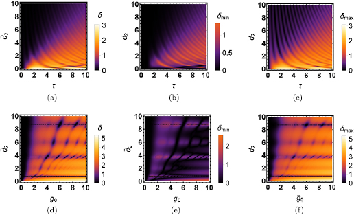
Figure 3. Non-Gaussianity of an optomechanical state with mechanical squeezing. In each row, the colours have been rescaled to correspond to the same values in the plot. The first row shows the non-Gaussianity as a function of time  and the squeezing parameter
  for the optical coherent state parameter and light–matter coupling
  and mechanical coherent state parameter
  . (a) Shows the full measure
  , (b) shows the lower bound
  , and (c) shows the upper bound
  . The non-Gaussianity generally oscillates in time and does slowly increase for increasing time
  . Furthermore, the upper bound
  approximates the full measure well for these parameters. The second row shows the non-Gaussianity
  as a function of the nonlinear coupling
  and the squeezing parameter
  for
for  and
and  at time
  . (d) shows the full measure
  , (e) shows the lower bound
  and (f) shows the upper bound
  . The non-Gaussianity increases with
  but decreases with
  .
.
Download figure:
Standard image High-resolution imageWe note that the non-Gaussianity increases for large light–matter coupling  and large coherent state parameter
  . This feature was also observed for standard optomechanical systems in [9]. However, the most striking feature here is that the larger
  is, the less non-Gaussian the system becomes. To understand why this is the case, we examine the dependence on
  in the function
  , since this determines the behaviour of the non-Gaussianity in certain regimes, as discussed in section 5.1. Using the expression (27) we find

For large  , and therefore large
  , the first term inside the brackets dominates and for
  with integer n, we are left with
  . In general, we find
  . The consequences for the non-Gaussianity are difficult to predict given the complexity of the expressions, but we note that the mechanical symplectic eigenvalue
  decreases, while the optical symplectic eigenvalue
  increases.
Furthermore, the quantity  is given by

We find that  . We then look at the symplectic eigenvalues (21) in this limit. We find that
  , and
, and  , which means that both the upper and the lower bounds of the non-Gaussianity tend to zero, and hence
  as
as  increases. We conclude that increasing the amount of constant squeezing in the system reduces the overall non-Gaussianity of the state.
5.3. Applications: modulated squeezing parameter
In this section, we consider a modulated squeezing term. The dimensionless squeezing  is time-dependent and of the form

where  is the amplitude of the squeezing and
  denotes the time-scale of squeezing13.
The differential equations in (12) are not generally analytically solvable for arbitrary choices of  . However, for the choice of
  in (30), both equations have a known form. Consider the differential equation for P11, which we reprint here for convenience,

Equation (31) is that of a parametric oscillator, which is used elsewhere in physics to describe, for example, a driven pendulum. As shown in appendix B, the equation for the integral of P22 (B.19) takes the same form.
The equation (31) is known as the Mathieu equation. In its most general form, and using conventional notation, it reads:

where  and x are real parameters. The general solutions to this equation are linear combinations of functions known as the Mathieu cosine
  and Mathieu sine
  , the exact form of which will be determined by the boundary conditions for y .
To find which values the a, q and x parameters correspond to, we note that the cosine-term in  has the argument
  , which means that we must rescale time
  as
as  . Inserting our expression for
  and using the chain-rule to change variables from
  to
to  , we rewrite the equation for P11 as

where we identify the variables  , and
, and  . The boundary conditions P11(0) = 1 and
  will yield the Mathieu cosine
  , and for
  as the solution, and the boundary conditions
  and
and  will yield the Mathieu sine
  as the solution. For our specific choice of
  in (30), the system is resonant at
  (see appendix E), which means that a = 1 and
  .
.
5.4. Approximate solutions at resonance
The Mathieu equations are notoriously difficult to evaluate numerically. Instead, we use a two-scale method to derive perturbative solutions to P11 and  . The perturbative solutions are valid for
  and make use of specific resonance conditions to ensure that the solutions do not diverge. See appendix E for the full derivation, where we also show that these approximate solutions correspond exactly to the more physically intuitive RWA when
  . For smaller values of
  , the approximate solutions are still valid, but they cannot be interpreted as equivalent to the RWA.
The squeezing term is resonant when  . We find that the approximate solutions for P11 and
  (the integral of P22) are given by, respectively,
We then compute  in (E.15). We assume that
  to find

where we have expanded the hyperbolic functions to second order. By using the relations between  and the Bogoliubov coefficients (B.30), we find that the Bogoliubov condition is approximately satisfied as:

With this expression, we can now compute the non-zero F-coefficients (9):
where we have discarded terms with  . With these expressions, we are ready to compute the non-Gaussianity of the system when the squeezing is applied at mechanical resonance.
5.4.1. Measure of non-Gaussianity at resonance.
We first compute the full measure of non-Gaussianity  and plot the results in figure 4. Figure 4(a) shows the full measure
  , the lower bound
  and the upper bound
  as a function of
  for the parameter
  ,
,  ,
,  , and
, and  as a function of time
  and the squeezing
  . The second plot in figure 4(c) also shows the full measure
  , the lower bound
  and the upper bound
  as a function of
  at
at  ,
,  ,
,  , and
, and  . We find that the non-Gaussianity increases with
  , as expected.
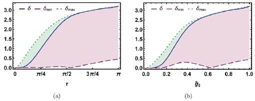
Figure 4. Non-Gaussianity of an optomechanical state with squeezing modulated at mechanical resonance. The plots show the measure of non-Gaussianity  together with its lower bound
  and upper bound
  . (a) Shows the non-Gaussianity as a function of time
  given the squeezing parameter
  , the optical coherent state parameter
  , the mechanical coherent state parameter
  , and the light–matter coupling
  . (b) Shows the non-Gaussianity as a function of
  at
at  ,
,  ,
,  , and
, and  . The upper bound
  approximates the full measure
  increasingly well as
  and
and  become larger.
Download figure:
Standard image High-resolution imageIn figure 4, we considered  ; a value consistent with the validity of the approximate solutions to the Mathieu equation. For this value, the non-Gaussianity is found to increase very slightly with
  . To demonstrate this, we consider the regime where
  , which occurs when
  for specific values of
  . In this regime, the non-Gaussianity was approximately given by
  (25). Given the functions (37), we find that

where we have again removed terms proportional to  and
and  . The behaviour of
  is markedly different compared with the constant case. Firstly, while
  still oscillates, it also increases with
  and
and  . If we consider the leading term with
  , we find that the non-Gaussianity scales with
  , which confirms that in this specific regime, the non-Gaussianity increases logarithmically with
  ,
,  , and
, and  . We conclude that squeezing is not necessarily detrimental to the non-Gaussianity if the squeezing is modulated at resonance, although more work needs to be done to ascertain the full interplay between the two effects.
6. Discussion
Before presenting our conclusions, we discuss the applicability and scope of the techniques we developed. We also comment on the effect of squeezing on the non-Gaussian character of the system.
6.1. Advantages over direct numerical simulations
With our techniques, we have shown that it is possible to analytically solve the dynamics of a nonlinear optomechanical system even when the mechanical squeezing is time-dependent. To emphasise this point, we wish to compare our approach, which relies on numerically solving the differential equations in (12), with a general numerical method using a standard higher-order Runge–Kutta solver to evolve a state in a truncated Hilbert space, e.g. using the Python library QuTiP [51].
When the dynamics is solved with a Runge–Kutta method, the continuous variable (pure) states are represented as finite-dimensional vectors in a truncated Hilbert space. When the system is nonlinear, information about the state is quickly distributed across large sectors of the Hilbert space. If the computational Hilbert space is too small, numerical inaccuracies quickly enter into the evolution, as a result of truncating the vectors. It follows that the dimension of the Hilbert space must be large enough to prevent this, which requires significant amounts of computer memory. It is also very difficult to consider parameters of the magnitude  and
and  , as done in this work, since these cause the system to evolve very rapidly and, consequently, require the evolution of the system to be calculated using smaller and smaller time intervals.
The methods developed here excel at treating systems numerically for large parameters  and
and  . However, we note that it becomes increasingly difficult to numerically evaluate the dynamics at longer times
  when the system of differential equation (12) is numerically solved for arbitrary functions
  . The difficulty is primarily caused by the double integral that determines the coefficient
  in (9), which must be evaluated numerically. For each value of
  , the integral will be evaluated from 0 to the final
  , and then from 0 to
  . As a result, the integrals take an increasingly long time to evaluate for large
  . We therefore conclude that the key strength in our method lies in evaluating the state of the system at early times
  for large parameters
  , and
, and  . We also emphasise that, the computation using our methods is numerically exact, which a naive computation using QuTiP or a similar library is not.
To conclude, our methods allow for the evaluation of the state of the system with large parameters, e.g.  and
and  , which would be nearly impossible to perform with QuTiP or a similar library unless one had access to significantly more computational resources.
6.2. Competing behaviours of nonlinearity and squeezing
We concluded from figure 3 that the addition of a constant squeezing term has a detrimental effect on the non-Gaussianity of the system. We also noted that inclusion of a constant squeezing term is equivalent to changing the mechanical trapping frequency  to a specific value and starting the computation with a squeezed coherent state (see appendix D). With this interpretation, our results also show that an initially squeezed state evolving under the optomechanical Hamiltonian can be expected to exhibit less non-Gaussianity compared with coherent states. The reason for this overall behaviour can be found by simple inspection of the total Hamiltonian. If a strong squeezing term is included in the Hamiltonian (1), it dominates over the interaction term, leading to a decrease in the non-Gaussianity. However, such a process is not fully monotonic, since an increase of the squeezing parameter does not always decrease the non-Gaussianity. This is, however, reasonable, as it cannot be expected that only the relative weight of the two parts of the Hamiltonian matter; the precise dynamics is much more complex, and the non-Gaussianity depends on the entire state, which is driven by the full Hamiltonian.
The finding that the non-Gaussianity increases with both time  and
and  when modulated at mechanical resonance is interesting and warrants further investigation. We leave this to future work.
7. Conclusion
In this work, we solved the time-evolution of a nonlinear optomechanical system with a time-dependent mechanical displacement term and a time-dependent mechanical single-mode squeezing term. We found analytic expressions for all first and second moments of the quadratures of the nonlinear system and used them to compute the amount of non-Gaussianity of the state. We considered both constant and modulated squeezing parameter, and found that a squeezing parameter modulated at twice the mechanical resonance results in the Mathieu equations, for which we provide approximate solutions equivalent to the RWA.
In general, we find that the relationship between the squeezing and non-Gaussianity is highly nontrivial. The inclusion of a mechanical squeezing term in the Hamiltonian, which is equivalent to starting with a coherent squeezed state evolving with the standard optomechanical Hamiltonian with a shifted mechanical frequency, decreases the overall non-Gaussianity of the state. If the squeezing term is modulated at twice the mechanical resonance, however, we found that the non-Gaussianity increases with both time and the squeezing parameter in specific regimes. These results hold interesting implications for quantum control of nonlinear optomechanical systems.
Our results also suggest that the combination of non-Gaussian resources and mechanical squeezing may not necessarily be beneficial if the application relies specifically on the non-Gaussian character of the state. However, more work is needed to conclude if this has a significant effect on, for example, sensing applications. More work is also necessary to properly study the instabilities of the full solutions to the Mathieu equations and how they affect the dynamics. The effect of squeezing the optical rather than mechanical mode is another question we defer to future work.
The decoupling methods demonstrated here constitute an important step towards fully characterising nonlinear systems with mechanical squeezing and can be used both to model experimental systems and to test numerical methods. The results presented here apply to any system with the same characteristic cubic Hamiltonian interaction term and single mode squeezing term. More broadly, the Lie algebra method can be used to solve any system where a finite set of Lie algebra operators has been identified. Our work can further be extended to more complicated quadratic Hamiltonians of bosonic modes, such as Dicke-like models [52], which would allow for applications in other areas of physics to be developed.
Acknowledgments
We would like to thank Antonio Pontin, Peter F Barker, Robert Delaney, Doug Plato, and Ivette Fuentes for useful comments and discussions.
SQ acknowledges support from the EPSRC Centre for Doctoral Training in Delivering Quantum Technologies and thanks the University of Vienna for its hospitality. DR would like to thank the Humboldt Foundation for supporting his work with their Feodor Lynen Research Fellowship. This work was supported by the European Union's Horizon 2020 research and innovation programme under Grant agreement No. 732894 (FET Proactive HOT). DEB acknowledges support from the CEITEC Nano RI.
Appendix A. Decoupling of techniques for time evolution
In this appendix, we outline the general decoupling techniques that we shall be using throughout this work to find a decoupled time-evolution operator generated by the Hamiltonian in (2).
A.1. Decoupling for arbitrary Hamiltonians
The time evolution operator  induced by a Hamiltonian
  reads
reads

Any Hamiltonian can be cast in the form  , where the
  are time independent, Hermitian operators and the gn(t) are time-dependent functions. The choice of
  need not be unique.
It has been shown [28, 47] that it is always possible to obtain the decoupling

where we have defined ![$ \newcommand{\e}{{\rm e}} \hat{U}_n:=\exp[-{\rm i}\,F_n(t)\,\hat{G}_n]$](https://content.cld.iop.org/journals/1751-8121/53/7/075304/revision2/aab64d5ieqn454.gif) and the real, time-dependent functions Fn(t), and the ordering of the operators is
and the real, time-dependent functions Fn(t), and the ordering of the operators is  .
.
The functions Fn(t) are uniquely determined by the coupled, nonlinear, first order differential equations

where  and all Fn are taken at time t. This is the general method we will be employing in the following sections.
A.2. Decoupling for quadratic Hamiltonians
If the Hamiltonian is quadratic in the mode operators the techniques described in the previous subsection have a more powerful representation. As explained in the main text, the time evolution operator has a symplectic representation  and the decoupled ansatz (A.2) has the form
  , where we have introduced
 ![$ \newcommand{\e}{{\rm e}} \boldsymbol{S}_n:=\exp[F_n(t)\,\boldsymbol{\Omega}\,\boldsymbol{G}_n]$](https://content.cld.iop.org/journals/1751-8121/53/7/075304/revision2/aab64d5ieqn459.gif) and the real, time-dependent functions Fn(t) are the same as those obtained with the technique above.
and the real, time-dependent functions Fn(t) are the same as those obtained with the technique above.
The real, time-dependent functions Fn(t) can be obtained by solving the following system of coupled nonlinear first order differential equations

where the matrix  can be obtained by
  and the summation is over
  terms [47]. This is the matrix version of the operator differential equation (A.3) for quadratic Hamiltonians, which reduces the problem of operator algebra to matrix multiplication.
Appendix B. Decoupling of the nonlinear Hamiltonian
We use the techniques presented in appendix A to decouple the Hamiltonian (2). The decoupling below is obtained in the same fashion of previous results in the decoupling of Hamiltonians [47, 49].
B.1. Solving the quadratic time-evolution
We start from the dimensionless Hamiltonian (2), which we reprint here

This Hamiltonian can be conveniently re-written as
Our goal now is to separate the Hamiltonian into a linear and a quadratic contribution. We then study the effect of the quadratic Hamiltonian on the nonlinear part, which allows us to focus fully on decoupling the nonlinear dynamics.
We therefore rewrite the time evolution operator (3) in the alternative form

where we have introduced

The transition to the expression (B.3) is similar to moving from the Heisenberg (or Schrödinger) picture to the interaction picture.
Our first goal is to solve the time-evolution of the quadratic part  . We define the basis vector
  . From standard symplectic (i.e. Bogoliubov) theory we know that

where the  symplectic matrix
  is the symplectic representation of
  and satisfies
  . Here
  is the symplectic form.
The matrix  therefore has the expression
 ![$ \newcommand{\e}{{\rm e}} \boldsymbol{S}_{\mathrm{sq}}(\tau)=\overset{\leftarrow}{\mathcal{T}}\,\exp[\boldsymbol{\, \Omega}\,\int_0^\tau\,{\rm d}\tau'\,\tilde{\boldsymbol{H}}_{{\rm sq}}(\tau')]$](https://content.cld.iop.org/journals/1751-8121/53/7/075304/revision2/aab64d5ieqn471.gif) . Here
. Here  and one has that

Therefore, we have that

It can be shown that the time independent orthogonal matrix  with expression

puts the Hamiltonian matrix  in diagonal form through

This allows us to manipulate (B.7) and find

This means that we have

We introduce the new vector  , which is just a rotation of the operators. Then we have

B.2. Solving the matrix time-ordered exponential
Here we seek a formal expression for (B.12). We write

in terms of the matrix  defined as

and the matrix  , which we will determine and which is diagonal. This follows from the fact that the matrix on the left-hand side of (B.13) is diagonal when squared, and therefore any even powers in the expansion will be diagonal. We use the fact that

to find the equation

Since  is invertible, we manipulate this equation and obtain, after some algebra,

We can now solve the four differential equations contained in (B.17) which read
The differential equation (B.18) must be supplemented by initial conditions. We note that since the left hand side of (B.13) is the identity matrix for  we have that
  which implies
  . In addition, taking the time derivative of both sides of (B.13) and setting
  implies
  .
.
By introducing the integral  , one can also rewrite the second equation as

so that it becomes the same as that for P11. The boundary conditions are now  and
and  .
.
We were not able to find a general solution to the differential equation for P11 (B.18) and the equation for  (B.19), but they can be integrated numerically when an explicit form of
  is given. For specific choices of
  , which we discuss in the main text of this work, the equations become the well-studied Mathieu equation.
Proceeding with the solution to the quadratic time-evolution, we have

In turn, this allows us to get

where we have introduced the Bogoliubov matrix  with coefficients
  and
and  .
.
This gives us, after a little algebra,
These quantities can also be written in terms of  as
as

This means that the basis vector  (B.5) transforms as

As a side remark, the Bogoliubov (symplectic) identities  read
read

B.3. Decoupling the nonlinear time-evolution
We can now go back to the time evolution operator (B.3) which we reprint here

Our work above allows to obtain

which can be conveniently rewritten as
Here we have introduced

for conveniency of presentation, where  and
and  are the real and imaginary parts of
  . Our definition of
  also implies that

We now note that the operators  form a closed Lie sub-algebra of the full algebra of our operators. Therefore, we can apply the decoupling techniques described above.
We proceed to decouple the remaining part of the operator (B.28), which reads

We make the ansatz

Taking the time derivative on both sides and arranging in a similar fashion to (A.3) we find

Therefore our main differential equations can be obtained by equating the coefficient of the different, linearly independent operators of the Lie algebra from the equation below
The solutions with operators proportional to  can be independently solved. However, the solutions for
  ,
,  , and
, and  are less straight-forward. We identify the following four coupled differential equations:

By first solving the equations for  and
and  , it is then possible to insert the solutions into the expressions for
  and
and  . We find the following key expression for this work

where  denotes the real part of
  and
and  denotes the imaginary part of
  . This result concludes the decoupling part of our work. The expressions (B.36), together with the decoupling form (B.32), can be used in the expression for
  (B.3) to obtain an explicit (up to a formal solution for
  ) time-evolved expression for the observables of the system.
Finally, let us once more write down the final expression of the time-evolution operator

to be complemented with the functions listed in (B.36).
Appendix C. First and second moments and covariance matrix elements
We can employ the results summarised in section 3 to compute all the relevant quantities needed in this work. They include the first and second moments of the state of the system at any moment in time, which we use to compute the measure of non-Gaussianity, see section 4. To do this, we use the explicit form of the time-evolution operator, written out above in (B.37). We further assume that the initial state is a separable coherent state ![$ \renewcommand{\ket}[1]{|#1\rangle} \ket{\mu_{{\rm c}}}\otimes \ket{\mu_{{\rm m}}}$](https://content.cld.iop.org/journals/1751-8121/53/7/075304/revision2/aab64d5ieqn515.gif) , defined in (15).
, defined in (15).
In order to compute the second moments that constitute the covariance matrix  for the state, we must calculate the expectation values of
  , and
, and  . To achieve this goal, we start by defining the following quantities for ease of notation:
and where we also introduce

which we use when deriving the state (16). The last two quantities can be computed using the expression for the Weyl displacement operator  and the combination
  , and read

The time-evolution of the operators  and
and  in the Heisenberg picture is therefore

These expressions allow us to compute the expectation values of the first and second moments given our initial state. We have here transformed into a frame rotating with  , which read

The two-mode covariance matrix is fully determined by its elements  , defined in this basis as
where all the other elements follow from the symmetries of  , imposed by the requirement that
  . Given all of the above, we can compute an explicit expression for elements (C.6) of the covariance matrix, which reads

C.1. Symplectic eigenvalues of the optical and mechanical subsystems
In this appendix, we use the covariance matrix elements to compute the symplectic eigenvalues of the optical and mechanical subsystems.
C.1.1. The optical symplectic eigenvalue.
We wish to compute the symplectic eigenvalue of the optical subsystem. It is given by

From the covariance matrix elements in (C.7) we find

By using the following trigonometric identities,
and from the fact that  , we obtain

Putting them together, we find

which can be simplified into
Next, we compute the mechanical symplectic eigenvalue.
C.1.2. The mechanical symplectic eigenvalue.
We first recall the Bogoliubov identities, which are  and
and  .
.
The mechanical eigenvalue is given by

Given the covariance matrix elements in (C.7), we find

This allows us to write

where we have suppressed the dependence of  for notational clarity.
We wish to simplify this expression by examining each term in turn and using the Bogoliubov conditions. We recall that

We can now use the Bogoliubov identities to show that

and

where we recall that  . Furthermore, we find

where we used  everywhere. We now note that the last term disappears because
  . We also note that
  is real, which follows from the Bogoliubov condition
  . When we take the real part, the second-to-last term disappears as well because it has an additional i, meaning that we are left with

We turn again to the symplectic eigenvalue, which we can now simplify as

Appendix D. Considerations of the scenario with constant squeezing
In this appendix, we show how a constant squeezing can be interpreted as a shift in the mechanical oscillation frequency  . The initial Hamiltonian (1) can be written as

where the quadratic part, which we call  , reads

To show how the squeezing affects the mechanics, we rewrite this as

where

This shows that  can be understood and implemented as a possibly time-dependent modulation of the frequency
  of the mechanical oscillator. For the case of constant squeezing
  , the Hamiltonian
  becomes time-independent and we can define
  and
and  with respect to
  such that

This transformation can be implemented by the squeezing operation  , where

which induces the mapping

When we apply this to the quadratic Hamiltonian, we obtain


To cancel the term proportional to  , we have to fix
 , and therefore,
  . With
  , we obtain

In particular,  under the replacement
  . Furthermore, we find that
  transforms as

When applying the same transformation to the nonlinear part of the Hamiltonian, we find

If  and
and  , which is indeed fulfilled for the interesting cases, we find that
  under the replacement
  , where

We define ![$\hat {H}_\mathrm{opt}^{\omega'_\mathrm{m}}:=\hat {H}_\mathrm{opt}[\omega_\mathrm{m}\rightarrow \omega'_\mathrm{m}]$](https://content.cld.iop.org/journals/1751-8121/53/7/075304/revision2/aab64d5ieqn558.gif) , and we obtain for the full time evolution
, and we obtain for the full time evolution

For the expectation values of quadrature of a state  , this leads to

where  . For the initial separable coherent state
  , we find that the time evolution of the quadratures induced by the full Hamiltonian
  with constant
  can be obtained by calculating the corresponding time evolution of the quadratures induced by
  with vanishing
  by replacing
  with
with  and considering the squeezed coherent initial state
  , where
  .
.
As a result, the techniques we have developed here can also be utilised to model all the expectation values for an optomechanical system for an initially squeezed states ![$ \renewcommand{\ket}[1]{|#1\rangle} \ket{\mathcal{D}_2(z)} $](https://content.cld.iop.org/journals/1751-8121/53/7/075304/revision2/aab64d5ieqn570.gif) .
.
Appendix E. Solutions to the differential equations at resonance
In this appendix, we first derive perturbative solutions to the Mathieu equations and then compare them with dynamics that we obtain from performing the RWA. We present two approaches which both amount to the same approximation while starting from different assumptions.
E.1. Approximate two-scale solution
Our goal is to obtain approximate solutions to the differential equations (B.18) and (B.19). We will do so by following the derivation in [53] with some modifications.
The general form of Mathieu's equation is given by

We will use the general notation in this appendix and then compare with the system in the main text.
We begin by defining a slow time scale X = qx. We then assume that the solutions y depend on both scales, such that  . This means that we can treat x and X as independent variables and the absolute derivative
  in (E.1) can be split in two:

Mathieu's equation (E.1) therefore becomes

We then expand the solution  for small q as
  and insert this into the differential equation above. Our goal is to obtain a solution for y 0 which incorporates a number of restrictions from the differential equation for y 1.
To zeroth order, we recover the regular harmonic differential equation for y 0, which is the limiting case as  :
:

where we know that the solutions are sinusoidal, while the coefficients must depend on X. We choose the following trial solution:

Our goal is now to find explicit solutions to the complex function  . We continue with the equation for y 1. We discard all terms of order q2 to find

We divide by q and insert our solution for y 0 to find

At this point, we specialise to a = 1, which corresponds to setting  in the main text. We combine the exponentials to find

In order for the solution to be stable, we require that secular terms such as resonant terms  vanish. If these do not vanish, the solution will grow exponentially [53]. We also neglect terms that oscillate much faster, such as
  . This leaves us with the condition that

which can be differentiated again and solved with the trial solution 
 for the parameters
  and c4. From the requirement in (E.9), it is now possible to fix two of the coefficients in (E.10). We differentiate
  and use (E.9) to find that the conditions
  and
and  must always be fulfilled.
We then recall that X = qx and after combining some exponentials, we obtain the full trial solution for the zeroth order term y 0:

We now proceed to compare this solution with the parameters and initial conditions given for P11 in (B.18) and  in (B.19) in the main text, which are both solved by the Mathieu equation.
First, we note that  and that
  . Then we consider the boundary conditions for P11, which are P11(0) = 1 and
  . From these conditions, we find that
  , and the the approximate solution to P11 is given by

The equation for  has the opposite initial conditions
  and
and  . For this case, we find that
  . The full solution to
  is therefore

and thus

Both solutions reduce to the correct solutions for the zero-squeezing case as  .
.
The validity of the pertubative approach can be determined as follows. By inserting the trial solution for  into the Mathieu equation, we are left with terms that are multiplied by
  . The leading term is in fact
  . These terms must be approximately zero to solve the Mathieu equation, which means that we require
  . This means that while
  , we can allow
  , which means that
  can be large provided that
  is sufficiently small.
From the expression for  in (B.29) we then find

For very small  , which was the condition for deriving the approximate solutions in the first place, we can approximate the fraction as unity and we find the compact expression

To better understand what this approximation entails physically, we compare it with the RWA, which has a well-known physical interpretation.
E.2. Alternative solution
There is another solution which more explicitly demonstrates how the resonance conditions helps constrain the solution. We write the solution to the differential equation for P11 as

Then, the differential equation  is solved approximately, considering only terms of first order in
  and neglecting terms rotating with frequency 3 off resonantly, by the following set of differential equations

These can be solved as

As the initial conditions for P11 are P11(0) = 1 and  , we find

which implies  , and
, and

The same steps as above can be applied to find an approximate solution for  :
:

with

and

which leads to

and

We find that

which exactly coincides with (E.15).
E.3. Comparison with the RWA
Here we compare the approximate resonance solution for P11 in (E.11) and  in (E.12) with the RWA, which is obtained as an approximation to the Hamiltonian in (1) when
  . In the main text, we separated the Hamiltonian (1) into a free term and a squeezing term (B.4), which for our specific choice of
  becomes

We now define the free evolution Hamiltonian  and the squeezing term
  as separate operators. We transform into a frame rotating with
 ![$ \newcommand{\re}{{\rm Re}} \newcommand{\e}{{\rm e}} \renewcommand{\dag}{\dagger}\exp[-{\rm i} \, \tau \, \hat{b}^{\dagger} \hat{b} ]$](https://content.cld.iop.org/journals/1751-8121/53/7/075304/revision2/aab64d5ieqn617.gif) , which means that the squeezing term transforms into
, which means that the squeezing term transforms into

For this specific case, the system becomes resonant when  . We can see this by expanding the cosine in terms of exponentials to obtain

When  , two of the time-dependent terms will cancel. We then perform the RWA, i.e. we neglect all remaining time-dependent terms. This approximation is only valid for
  . In the interaction frame, we find

In the symplectic basis  the corresponding symplectic operator, given by
  , where
  and
and  is given by

The symplectic representation of the squeezing operator (B.7) in the lab frame reads

where  encodes the evolution from the Hamiltonian
  . We therefore find the Bogoliubov coefficients

which evidently satisfy the Bogoliubov conditions, and obtain

This expression exactly matches the one we derived as a perturbative solution to the Mathieu equations in (E.15). However, the requirement for the validity of the RWA is that  , while the approximate solutions are still valid for small
  . We conclude that the approximate solutions only coincide with the RWA for large
  , while this interpretation cannot be used when
  .
.
Footnotes
- 9
We note here that non-Gaussianity for the case
has been already studied [9]. - 10
Note that
is complex in our choice of basis, which implies taking the Hermitian conjugate of . - 11
For example,
or , where the numbering and ordering of the generators is a matter of convenience. Work in this direction has also been done in [48]. - 12
In particular, the Hamiltonian (2) is generated by a linear combination of the Hermitian operators
, , , and . - 13
We remind the reader that our rescaled quantities require us to use
and we define .


