

Abstract
In this work we investigate how regular islands localized in a mixed phase-space of generic area-preserving Hamiltonian systems are affected by a small amount of dissipation. Mainly we search for a universality (hierarchy) in the convergence of higher-order resonances and their periods when dissipation increases. One very simple scenario is already known: when subjected to small dissipation, stable periodic points become sinks attracting almost all the surrounding orbits, destroying all invariant curves which divide the phase-space in chaotic and regular domains. However, performing numerical experiments with the paradigmatic Chirikov–Taylor standard mapping we show that this presumably simple scenario can be rather complicated. The first, not trivial, scenario is what happens to chaotic trajectories, since they can be attracted by the sinks or by chaotic attractors, in cases when they exist. We show that this depends very much on how basins of attraction are formed as dissipation increases. In addition, we demonstrate that higher-order resonances are usually first affected by small dissipation when compared to lower-order resonances from the conservative case. Nevertheless, this is not a generic behaviour. We show that a local hierarchical collapse of resonances, as dissipation increases, is related to the area of the islands from the conservative case surrounding the periodic orbits. All observed resonance destructions occur via the bifurcation phenomena and are quantified here by determining the largest finite-time Lyapunov exponent.
Export citation and abstract BibTeX RIS
1. Introduction
It is well known that the behavior in conservative and dissipative systems is completely different. The phase-space of typical nonlinear conservative systems can present regions of regular, chaotic and mixed (coexistence of regular and chaotic) motion, depending on the nonlinear parameter strength. Specifically, for two-dimensional Hamiltonian area-preserving maps, chaotic and regular motions are clearly separated by KAM (Kolmogorov, Arnold and Moser) [1] curves which prohibit chaotic orbits to penetrate the regular domains or even to reach all points in phase-space. The behavior of chaotic trajectories in the mixed motion can be very complicated, including a kind of intermittent behavior, spending a long time sporadically near the border of regular islands [2, 3]. Such sticky motion, even close to tiny regular islands, can exert an expressive influence on the global dynamics [1, 4, 5], which is completely different from what occurs in hyperbolic systems. In this context, a significant number of studies in the literature characterized the existence and the effect caused by such regular islands in the dynamics of conservative systems [1, 5–14].
In complete distinction to the above cases, dissipative systems arbitrarly near to the overdamp limit, can present few or only one attractor to which all initial conditions eventually converge, because its basin of attraction usually occupies a considerable portion of phase-space [15]. However, from the physical point of view, conservative and dissipative systems are not completely independent and in some problems the transition from one to another occurs during a continuous change of parameters [16, 17]. In such cases there exist an intermediate regime, very close to the conservative limit, where the dynamics can be intermixed resembling both conservative and dissipative features. Usually, the characterisation of such features represent a hard task and are related to the regular islands that become island sinks or just sinks when dissipation is taken into account in conservative systems [18]. In a more general context, conservative systems coupled to high-dimensional environments become weakly dissipative and may exhibit chaotic behaviour in this transition [19].
In this work we analyze the effect of including a small amount of dissipation via the damping constant which multiplies the momentum variable in a typical area-preserving mapping model, namely the Chirikov–Taylor standard mapping [20], defined in next section. The main physical motivation is based on the fact that small dissipation is inevitable in real systems and its influence on the dynamics of conservative Hamiltonian systems is of great interest. Stable periodic points become sinks attracting many rational/irrational curves localized in the their neighborhoods and all KAM curves are destroyed [21–23]. Small dissipation in mixed dynamics induces a transient chaotic motion and the time after which the chaotic trajectory is attracted to a sink can be measured [1, 21]. Such persistent chaotic motion is densely interwoven with regular motion making the dynamics very complex [24] due to the huge amount of attractors which exist [25–28] in the weak dissipative limit. Therefore, it is very hard to tell a priori to which attractor trajectories will converge. In other words, considering the presence of an arbitrary small amount of dissipation in a typical conservative system one would like to know if some hierarchical destruction of regular islands or born of attractors exist. Under increasing dissipation, we present numerical and analytical results about the phase-space deformation, convergence (collapse) of trajectories to some attractor and use the largest finite-time Lyapunov (FTLE) to detect changes of stability suffered by periodic orbits. With these results we try to elucidate how arbitrary small dissipation affects the regular islands in the transition from the conservative to dissipative regime. Our main findings suggest that higher-order resonance islands found in the phase-space of area-preserving maps are the first affected and destroyed by dissipative effects. However, there is apparently no hierarchical collapse regarding the periods of the orbits. A local hierarchy of collapses,  , was found for the examples discussed here.
  estimates the priority of a period-p stable orbit to collapse to another stable attractor as the dissipation parameter γ increases.
  is the area of the islands from the conservative limit surrounding the corresponding period-p point. Large values of
  implies priority in the sequence of collapses and reveals a hierarchy.
The paper is organized as follows. In section 2 the dynamical system used in our study is introduced. While in section 3 some analytical properties of tori under dissipation are presented, section 4 discusses the numerical results in detail. Finally, in section 5 we summarize our main conclusions.
2. The discrete time model
Based on the well known Chirikov–Taylor standard mapping [20], considered a prototype model for chaos and quantum chaos studies, we introduce a dissipative version for this map as proposed in [29], which is defined as

where K is the nonlinearity parameter and ![$(x_n, p_n)\in [0, 1]$](https://content.cld.iop.org/journals/1751-8121/51/10/105101/revision2/aaaaabdieqn005.gif) are canonical conjugated variables of generalized action and phase, evaluated at discrete times
are canonical conjugated variables of generalized action and phase, evaluated at discrete times  .
.  is the determinant of the Jacobian matrix of the map, where γ is the dissipation parameter which reaches the overdamping limit for
  and conservative limit for
  . It is well known that the period-1 (shortly written per-1 along the text) fixed points are p1 = 1/2m (m integer) and
  . The point x1 = 0 is always unstable while
  becomes unstable for K > 4. There exist also per-1 fixed points related to accelerator modes [20], whose stability condition is
  , with
  and l integer. For higher periods there are primary families of periodic points (which exist in the limit
  ) and bifurcation families which are born only for larger values of K. A detailed discussion about the bifurcation process can be found in [1] and [11] for the dissipative and conservative regimes, respectively. Specifically in this work, the numerical simulations was performed keeping the nonlinearity parameter fixed as K = 2.5.
3. Tori under small dissipation: analytical results
The dissipation introduced in (1) follows from a damping term usually written as  , where p is the particle's momentum. For a more general understanding about the effects of such dissipation model, it is interesting to analyze how tori and separatrix from the conservative case are changed when adding dissipation. In low-dimensional conservative systems the origin of chaotic motion comes from the motion close to the separatrix. However, for the cases considered in this work, the perturbation parameter K from (1) is so large that the separatrix is already destroyed and it makes no sense to discuss it here.
3.1. The dissipative twist map—the linear case
The effect of dissipation on tori can be nicely described using the dissipative twist map


where ( ) may represent canonical variables. The Jacobian of the above map is equal to J. Therefore, for J = 1 the above map is the conservative twist map [1]. Here
  with
with  being the rotation number. For J = 1 the dynamics obtained from (2) and (3) is a rational torus when
  assumes a rational value k/q, with k and q being integers. In such cases a rational torus with period-q is obtained. For irrational values of
  , the dynamics is an irrational torus. The map (2) and (3) allows us to understand the basic general effect of our dissipative model acting on rational/irrational tori from the conservative case. Similar dissipative effects on the rational and irrational tori are expected for the dynamics of the map (1).
The explicit time evolution of the variables ( ) can be obtained by applying the discrete Laplace transform [30] in equations (2) and (3)


After long but straightforward calculations which involve partial fractions decomposition of the coefficients for the inverse Z-transform evaluation, we obtain:

The angle θ is defined through:


where we introduce factor 1/(2J1/2) such that  . Thus,

being  and
and  . For one numerical example we use
  ,
,  and J = 0.8 to plot in figure 1 the iterations of maps (2) and (3) together with analytical solutions given by equations (6) and (7).
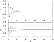
Figure 1. Time series for x and y of the map given by equations (2) and (3) (red dots). The analytical solutions obtained throught the Z-transform and given by equations (6) and (7) are also depicted (black continuous lines). Here the parameters are chosen such that  , with initial conditions x0 = 0.1 and y0 = 0.21.
Download figure:
Standard image High-resolution imageThe analytical solutions show that dissipative effects destroy the tori, and they collapse from ( ) to (0,0) with a time decay proportional to
  . For 0 < J < 1, which is the case of dissipation,
  and the decay becomes proportional to
  . Thus, the dissipative model used here induces an exponential convergence in time. However, for tiny dissipation this decay can be very slow, in fact linear. This can be checked by expanding the exponential in a Taylor series around
  . As an example, using J = 0.999, after n = 1000 iterations we have
  , and for J = 0.99 we have
  for the same number of iterations. Results from this section are applied for rational and irrational tori.
3.2. Dissipation close to non-linear resonances
In area preserving mappings, by slightly perturbing a two-dimensional integrable system, it is possible to obtain a perturbed twist mapping [1]. By conveniently linearizing such a map around a fixed point the result is the standard map (1) with K essentially proportional to  [5] and J = 1. Here
  is the perturbation parameter, V0 is the perturbation calculated at the resonance condition and k0 is the order of the nonlinear resonance. This means that any attempt to understand the effect of dissipation in the presence of nonlinear resonances can use map (1) with
  and
and  . To check this, figure 2(a) demonstrates the convergency of the interpolated radius
  for one initial condition and K = 0.1, for which the map (1) has only one fixed point at
  . Black for J = 0.9999, red for J = 0.9995, green for J = 0.999, blue for J = 0.995 and yellow for J = 0.99. In these cases the exponential decay
  has β given respectively by
  ,
, 
 ,
,  and
and  . In figure 2(b) we use K = 2.5 (same values of J) to describe the results regarding higher order resonances discussed in section 4.4. In these cases β is given respectively by
  ,
,  ,
,  ,
,  and
and  .
.

Figure 2. Time series for radius rn of the map (1) for (a) K = 0.1 with ICs  and (b) K = 2.5 with
  .
.
Download figure:
Standard image High-resolution image4. Numerical results
4.1. Deforming the conservative phase-space: the role of dissipation
We start this section discussing the general behaviour of stable and unstable periodic orbits when arbitrary small dissipation is considered. Figure 3(a) shows the phase-space for the conservative case ( ). The two per-1 stable points, also known as primary resonances, are localized at p = 0 (see the red line in figure 3(a)) with
  . The four stable elliptic points, or secondary resonances, related to the per-4 orbit are located at p = 0,
  and
and  ,
,  , which can be seen figure 3(b), which is an amplification of the domain delimited by a red box drawn in the upper-left part of figure 3(a). These secondary resonances are surrounded by their corresponding rational/irrational tori and also by some smaller elliptic points, the ternary resonances and so on. Since the set of stable points related to the primary and secondary resonances will be discussed in more detail later, we introduce the notation
  and
and  , respectively. The sign refers to the sign of x, or the location of the stable points, i.e. left for negative and right for positive x values. Moreover, as some specific periodic orbits will be further investigated in the section 4.3, we also define the notation
  and
and  , where the sign and subscript-index have the same meaning introduced in the last sentence, while the superscript-index τ is the period of the orbit which will be discussed later. For example,
  refers to the point of a periodic orbit with period 28, which is located around the main island with period-4. The remaining phase-space dynamics is chaotic, beside some tiny stable points, not visible in the resolution shown.
Figure 3. (a) Phase-space plot ( ) for K = 2.5,
  , and 200 ICs chosen uniformly along the red-line at p = 0. (b) Amplification of a red box around the upper-left island of period 4. (c) Same phase-space plotted as in (a) but now under dissipative effects setting
  .
.
Download figure:
Standard image High-resolution imageThe domains with regular motion are not stable under dissipative perturbation. By adding an arbitrary small amount of dissipation to the dynamics,  for instance, we observe in figure 3(c) that rational/irrational tori are destroyed and the stable points become attracting centres or sinks [21, 22]. In other words, we can say the tori lose their energy and converge to the stable elliptic point they belong to. This is a very typical behaviour in the conservative to dissipative transition, also shown analytically in section 3. While elliptic points are transformed into sinks and surrounding orbits converge to it, chaotic orbits usually converge to the chaotic attractor. In other words, we can say that the phase-space near to the conservative limit is dominated by periodic attractors with different periods [25–27], where stable points or resonances become attractors and tori are destroyed giving rise to the basin of attraction. Roughly speaking, when slowly increasing the amount of dissipation in the system, points on the tori become basins of attraction for the periodic points and the chaotic motion is replaced by a very long chaotic transient motion that occurs before the trajectory converges to the chaotic attractor. The asymptotic state of system is extremely susceptible to transient behaviour.
In fact, even though the above behaviour seems to be simple, it is not. We have to remember that this is the origin of the basin of attraction in dissipative systems which has complicated and fractal structures [15]. The border line between the basin of attraction for distinct attractors is an invariant line. For small dissipation the stable irrational tori surrounding the elliptic points apparently just converge to their corresponding elliptic point. However, what happens to higher-order resonances which live at the border between irrational tori and the chaotic motion? We remember that each higher-order resonance has its own surrounding irrational tori. We can also ask what decides if a chaotic trajectory from the conservative case converges to one specific elliptic point, or to a fractal attractor as dissipation increases? These are some of the important questions that we discuss in this work.
We start analyzing how one irrational torus is deformed by different dissipation intensities. For this we plot figure 4, which is a magnification of the box drawn in figure 3(a), for different values of γ. Figure 4(a) presents the conservative case ( ) and the red curve is the KAM torus generated by the initial condition
  , chosen in the neighborhood of a stable point localized at
  . Setting
  , the main visible effect is that the torus becomes thick, as seen in figure 4(b). In this case, the dissipation is not strong enough to allow the perturbed torus to break and converge exactly to the nearest stable point labeled
  . Although the trajectory is closer to
  when compared to the torus from the conservative case. Increasing dissipation to
  the orbit is completely broken and converges to a point apart from
  , as shown in figure 4(c). Increasing the dissipation more (figure 4(d)) makes the convergence become faster and the trajectory is attracted by the sink (attractor) at
  , which is the point
  from the conservative case.

Figure 4. Black dots and lines are magnifications of the phase-space plot ( ) with K = 2.5 and
  . (a) Red curve (
 ) obtained with only one initial condition:
  , while red points represent the position of the attractor generated from the same curve when (b)
  , (c)
, (c)  , and (d)
  .
.
Download figure:
Standard image High-resolution imageAnother way to see the importance of dissipation is by looking at figure 5, where in (a) and (b) we display the phase space dynamics for the same values of γ used in figures 4(c) and (d), namely  and
and  , respectively. In figure 5 (a) there are six regions with a higher-density of points when compared to the rest of the phase-space. These regions are close to the stable points
  and
and  from figure 3(a), which are now transformed into attractors. Increasing the values of the dissipation, figure 5 (b) shows that the higher-density of points are now close to
  , a consequence of the fact that
  became unstable. Consequently, all attractors generated with higher-order resonances converge, due to dissipation, to attractors associated to primary resonances. Figures 5(a) and (b) can be compared to figure 3(c), where the dissipation is smaller and the density points increase also around higher-order resonances, the behaviour of which is explained next.

Figure 5. Phase-space plot ( ) for K = 2.5, and 200 ICs chosen uniformly along the red-line at p = 0 in figure 3(a) and (c) for (a)
  and (b)
  . (c) Asymptotic or final position (xf) in the phase-space as a function of dissipation γ for two initial conditions, one close to the per-4 fixed point
  and the other one at the per-
 orbit from figure 3(b).
Download figure:
Standard image High-resolution imageFigure 5(c) displays the final orbital location (xf) as a function of γ. To obtain this picture we use two ICs, one at  (black curve), localized near to the stable point
  , and the other one (red curve) at
  , related to the per-
 from figure 3(b). With these ICs the standard map was iterated 104 times for 200 values of the dissipation parameter in the range
 ![$\gamma=[0:1]$](https://content.cld.iop.org/journals/1751-8121/51/10/105101/revision2/aaaaabdieqn100.gif) . For each value of γ distinct xf are reached. Close to
. For each value of γ distinct xf are reached. Close to  the per-
 around the island from figure 3(b) collapse together with the black curve, which is related to the IC from the stable point
  . Thus, for
  the per-
 disappears. For
  , both trajectories converge to the point related to
  .
.
Summarizing this part, we conclude that when a small amount of dissipation is introduced in conservative systems, tori around an elliptic point are destroyed, becoming points which belong to the basin of attraction of this elliptic point, which is now an attractor. For tiny dissipation the number of attractors should be equal to the number of resonances from the conservative case, which can be huge. As dissipation increases, attractors related to higher-order resonances are destroyed first, leading to a hierarchy of the destruction of attractors. For strong dissipation, only primary resonances tend to survive. With these results we are tempted to conclude that the hierarchy of convergences, as dissipation increases, follows the simple rule: higher-order resonances converge to lower order resonances and so on. However, as we will see next, the hierarchy follows a more complicated scheme.
4.2. Dynamics dependence on initial conditions and dissipation strength
When adding weak dissipation, it is very difficult to know in general to which attractor a given IC belongs to. Besides the ICs on the torus close to the elliptic points, all other points in the phase space can belong to a distinct basin of attractions. In this section we study this in more detail. In figure 6 we plot the initial position versus convergence point ( ) after n = 104 iterations, considering the interval x0 = [−0.5:0.5], and four distinct values of dissipation. Starting with figure 6(a), where
  , we can clearly identify the ICs chosen in the neighborhood of some stable point (from the conservative regime) converging to itself. For example, the IC
 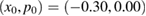 , which is inside the regular island close to
  , generates a trajectory that converges to xf = −0.32, as indicated by the blue-dashed line. A similar behaviour occurs for other ICs, chosen close to a lower resonance, as can be seen for xf = −0.50, and indicated by the red-dashed line. This is the location of the largest regular island where the stable point
  exists. Otherwise, initial values of x0 chosen outside the regular islands are related to the chaotic asymptotic behaviour. Such behaviours become much more evident as dissipation increases, as can be seen in figures 6(b)–(d). For
  , we see in figure 6(c) that ICs inside the regular islands around
  converge to
  , while ICs started inside the islands related to stable points
  , converge to
  . However, when dissipation increases to
  , we clearly see in figure 6(d) that all ICs chosen inside any regular island converge to the same final point xf = +0.50 or −0.50.
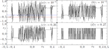
Figure 6. Convergence point xf as a function of initial position x0 for K = 2.5 along the line p0 = 0, (a)  , (b)
, (b)  , (c)
, (c)  , (d)
, (d)  .
.
Download figure:
Standard image High-resolution imageThe dependence of xf over the choice of initial position x0 can be nicely explored using a mixed-plot, which was proposed recently to describe generalized bifurcation diagrams [11]. Figure 7 displays the mixed-plot, where red, yellow to white colours indicate increasing positive values of xf, and cyan, blue to black colours belong to increasing negative values of xf. ICs are taken along the line p0 = 0 and x0 = [−0.5, 0.5]. Near the conservative limit ( ), the rational/irrational tori and the chaotic trajectory surrounding the stable points
  and
and  converge respectively to these points. See for instance, that the rational/irrational tori surrounding
  converge to
  , which are the white (represented by sign +) and black (represented by −) points. Rational/irrational tori surrounding
  , and ICs inside the chaotic domain, converge to
  , and are related to yellow for + and blue for − convergence points. Moreover, the ICs chosen in the chaotic domain, between the regions associated to
  and
and  , converge to other points in the phase-space, probably to the chaotic attractor. This can be recognized by the mixture of colours designed for xf in figure 7(a). As dissipation increases, we see the evolution of the final points xf. For
  , the stable points
  do not attract the surrounding tori anymore (yellow and blue points around these points disappear). The corresponding ICs now converge to the points
  represented by white and black colours. The large variety of colours for xf also start to disappear, but in a complicated and intricate way. For stronger values of dissipation all the ICs converge to the points
  , which are the points remaining from the primary resonances in the conservative limit. Figure 7(b) illustrates very well the complex scenario we found. It is a magnification between chaotic and regular ICs, which is a portion of figure 3(a) between the points
  and
and  . The larger yellow stripe is reminiscent of ICs from the conservative case which were close to the border of the last tori around
  [a similar (blue) stripe exists for
  ]. Please observe that the yellow stripe starts for
  at the border of the large yellow stripe from figure 3(a). All these ICs start close to
  .
.
Figure 7. (a) The convergence point xf is plotted (in different colours) as a function of the dissipation parameter γ versus the initial position x0 along the line p0 = 0 for K = 2.5. (b) Magnification of the red box shown in the top panel.
Download figure:
Standard image High-resolution image4.3. Characterizing stability changes using the largest finite-time Lyapunov exponents
The third strategy used to study the hierarchical destruction of regular islands is based on the application of the largest finite-time Lyapunov exponents (FTLEs). It will help us to check if there is a stability change when ICs change their attractor due to small dissipation. Since our interest is related to the study of the convergence properties of stable orbits under dissipative effects, the largest FTLEs, represented by λ, has negative values and becomes zero at the bifurcation points. For more details about the application of this method to study conservative systems we refer the readers to see [11]. From the numerical point of view we calculate the FTLEs using Benettin's algorithm following [31] and [32], which includes the Gram–Schmidt re-orthonormalization procedure.
We start calculating numerically the FLTEs as a function of the iteration time n for one initial condition,  chosen inside the regular island around
  , and for three different values of dissipation parameter:
  (black curve), 10−4 (red curve) and 10−3 (blue curve). The results are plotted in figure 8(a), where the straight horizontal line displays the value zero, for reference. The black curve (i) is the conservative case where λ tends to zero, as expected for stable periodic orbits in conservative systems. This convergency to zero can be checked for longer times in the log–log plot in the inset of figure 8(a). As dissipation increases to 10−4 the convergence of
  in the blue curve (ii) is faster. Around
  iterations λ crosses the zero line and becomes slightly negative. For 10−3 this convergence, observed by the red curve (iii), is even faster and λ becomes more negative. Other values of γ were checked and the main behaviour described in figure 8(a) remains practically unchanged.
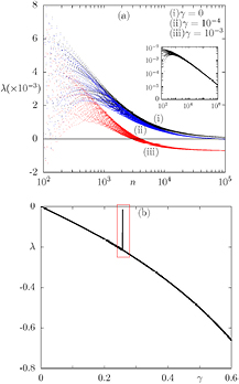
Figure 8. Largest FTLEs (a) as a function of iteration time for three different values of γ and (b) as a function of dissipation obtained for 105 iterations. In both figures K = 2.5 and p0 = 0. The inset in (a) shows the log–log plot of the  case for longer times.
Download figure:
Standard image High-resolution imageNow we calculate the FTLEs as a function of the dissipation parameter for the same IC used to obtain figure 8(a) and plot the result in figure 8(b). For  we have
  , as expected for the conservative case. When the dissipation parameter slowly increases, λ becomes more and more negative in agreement with the results from figure 8(a). For
  a peak in the value of λ is observed inside the red box drawn in figure 8(b). At the peak, the FTLE is close to
  suggesting that for
  a bifurcation occurs. This is apparently the case. We remember that
  is approximately the dissipation value for a discontinuity (or a 'jump', or 'collapse' of attractors) in the convergence point xf (plotted in figure 5(c)). In other words, for values of
  , trajectories are not attracted to
  anymore, but they start to converge, via a bifurcation procedure, to the attractor at
  . Thus, there is a switch of attractors via the bifurcation phenomena.
4.4. Collapse of higher-order resonances
The goal of the present section is to make a systematic analysis of the collapse of higher-order to lower-order resonances as dissipation increases. For this we choose seven exemplary periodic orbits shown in figure 9(a). To better identify such orbits, for each periodic orbits we plot one surrounding irrational torus with a given colour. Forest-green around periodic point  , cyan around
  , olive around
  , dark-red around
  , blue around
  , thick black around
  and dark-violet around
  . The choice of these periodic orbits is appropriate to analysing two main questions: (a) to which attractor and (b) in what order these orbits will collapse as dissipation increases? Notice that all periodic orbits are surrounding one of the
  fixed points. However, there is an important distinction between them. While periods
  and
and  are trapped to
  by some external torus (see dark-orange torus), orbits
  and
and  are, naively speaking, free to be attracted to the external chaotic regime when dissipation increases. However, this is not what occurs, as shown for the orbit
  in figure 9(b). This periodic orbit (
 ) is originally generated by the IC
  for
for  . As dissipation increases, the
  orbit survives until
  , where a bifurcation (FTLE close to zero) phenomenum occurs and it collapses directly to the
  point. Thus, it does not collapse to an intermediate higher-order resonance. In fact, from the seven chosen periodic orbits, this is the only one which collapses to
  , all other five orbits collapse, as dissipation increases, directly to
  . This answers question (a), that there is apparently no way to predict exactly to which attractor higher-order resonances will collapse. In order to answer question (b) we determine the sequence, as dissipation increases, for the collapse of the periodic points directly to
  . This is summarized in table 1 (please note that period
  is not shown since it did not collapse to
  ). The first row shows the periods of the orbits and the second row the values of γ for which these orbits collapse to
  . There is no evident collapse hierarchy observed in the periods of the orbits. However, a nice relation is observed when we compute the area
  (third row) of the islands from the conservative case surrounding each stable point. For example, the island surrounding the period
  in figure 9(a) is much larger than the island surrounding period
  . We found that the period
  is more stable under dissipation than
  (see table 1). This suggests a relation between the values of γ where collapses occur and the mentioned area. To approximately determine these areas we performed additional simulations (not shown) and estimated them directly from the phase space, in arbitrary units. We only considered the area around one orbital point from each periodic orbit. For tiny areas such as
  and
and  , we could not obtain reliable precision to distinguish them. Table 1 shows a direct relation between the increasing values of γ and the increasing values of
  . Therefore, the collapse of a periodic point under dissipation is proportional to the size of the island from the conservative limit surrounding these points. In other words, the collapse to
  is inversely proportional to
  . The same results should be valid for
  . In addition, it is also clear that the same hierarchy occurs for the collapse of periods
  and 4 to
  . More generally, we may conjecture that
  , where
  estimates the local collapse priority of a period-p stable orbit as dissipation increases and
  is the area of the island from the conservative limit surrounding the corresponding periodic point.

Figure 9. (a) Magnification of phase-space from figure 3(b). Some tori are plotted in colour to better identify the corresponding periodic orbits. Forest-green tori around periodic point  , cyan around
  , olive around
  , dark-red around
  , blue around
  , thick black around
  and dark-violet around
  . (b) Convergence or final position xf as a function of dissipation near the transitions between attractors, namely
  (c) FTLEs of the periodic orbits from panel (b) plotted versus dissipation, characterizing the exact point where the trajectory change of attractor.
Download figure:
Standard image High-resolution image
Table 1. Values of γ for which the stable attractors with period-p collapse to  .
.  is the area, in arbitrary units, of the islands from the conservative case around the periodic point with period-p.
| Period-p |  |
 |
|---|---|---|
 |
 |
0.07 |
 |
 |
0.07 |
 |
 |
0.64 |
 |
 |
3.99 |
 |
 |
13.3 |
5. Summary and conclusions
In summary, we have studied the behavior of conservative trajectories submitted to weakly dissipative effects. This class of problems has interesting applications e.g. for the break of time symmetries creating appropriate conditions for the existence of ratchet currents [33–36], and the prevention of unlimited Fermi acceleration [16, 37], or the induction of anomalous transport due to random perturbation [24], among others. Our main interest in this work is the analysis of how the dynamics of a generic Hamiltonian area-preserving map, namely a Chirikov–Taylor standard map given by equation (1), is modified as dissipation increases starting from the conservative limit along the line p0 = 0. When tiny dissipation takes place, a huge (but finite) number of periodic attractors are created and they are responsible by the complex behaviour associated with multistability. In this scenario, the convergence properties of the stable and unstable trajectories are strongly affected by the local hyperbolicity in the interface between the regular and chaotic domain, as presented in [38]. This behaviour is one of the most important reasons which motivated us to perform the present investigation.
The main results obtained in this work can be presented in three different sets of conclusions associated to dissipation intensities: (i) For tiny values of γ quasi-periodic orbits from the conservative regime tend to be attracted to their corresponding stable periodic point. However, with counter examples we showed that this is not a generic rule. (ii) As dissipation increases, higher-order resonances and their surrounding quasi-periodic motion from the conservative limit tend to collapse to lower-order resonances. However, a resonance with order p may collapse to a q-resonance (p > q) before a k-resonance (k > p) collapses to the same q-resonance. Specifically, this result shows that there is no visible hierarchy of collapses concerning the period of resonances presented in phase space. However, a hierarchy of collapses in subdomains composed of primary and specific higher order resonances was found regarding the area of islands from the conservative case surrounding the periodic point. From our numerical observations we propose the conjecture that  . Here Hp estimates the priority of collapse of a period-p stable orbit as dissipation increases and
  is the area of the island from the conservative limit surrounding the corresponding periodic point. Certainly this result deserves future investigation. (iii) For strong dissipation all trajectories are identically attracted by attractors generated from the period-1 islands of the conservative limit. Based on these conclusions, we can see that when a sufficiently small amount of dissipation is considered, the distribution of state points in phase space become non-uniform, similar to what happens in mixed Hamiltonian phase spaces, i.e. sub-sets in phase space present distinct dynamical behaviour. We believe these results give essential hints and open questions for further investigation on the effects caused by small amounts of dissipation added to typical Hamiltonian systems. Future work on this subject may include the computation and analysis of stable and/or unstable manifolds around fixed points as dissipation increases, as done for unstable fixed points [39].
Acknowledgments
The authors thank CNPq and CAPES (Brazilian agencies) for financial support. C M also thanks FAPESC (Brazil) for financial support.