

Abstract
We study a self-dual generalization of the Baxter–Wu model, employing results obtained by transfer matrix calculations of the magnetic scaling dimension and the free energy. While the pure critical Baxter–Wu model displays the critical behavior of the four-state Potts fixed point in two dimensions, in the sense that logarithmic corrections are absent, the introduction of different couplings in the up- and down triangles moves the model away from this fixed point, so that logarithmic corrections appear. Real couplings move the model into the first-order range, away from the behavior displayed by the nearest-neighbor, four-state Potts model. We also use complex couplings, which bring the model in the opposite direction characterized by the same type of logarithmic corrections as present in the four-state Potts model. Our finite-size analysis confirms in detail the existing renormalization theory describing the immediate vicinity of the four-state Potts fixed point.
Export citation and abstract BibTeX RIS
1. Introduction
Once upon a time, the idea originated [1] that marginally irrelevant scaling fields can introduce logarithmic corrections to scaling. The two-dimensional, four-state Potts model, for which some exact analysis is possible [2], is a celebrated example of this kind of behavior. Cardy [3] investigated the presence of such corrections to the finite-size scaling behavior of this model. If we denote by v the marginal field, and by L the linear dimension of the system, Cardy considered the effects of multiplicative logarithmic correction factors of the form ![$c_k v^k/[1-v\ln(L)/\pi]^k$](https://content.cld.iop.org/journals/1751-8121/50/32/324001/revision2/aaa7b53ieqn001.gif) . His approach assumed that
. His approach assumed that  and
and  , so that the v-dependence vanishes to lowest order of
  . The numerical data upon which Cardy's based his analysis were obtained from transfer-matrix computations for strips of a limited range of widths L [4], and his analysis was predicated on the assumption that
  was sufficiently large.
In this paper we study a generalized Baxter–Wu model in which that condition is not always satisfied. As a matter of fact, in our case  can be made arbitrarily small, as discussed in greater detail in section 2. Our purpose is to verify the precise form of these logarithmic correction factors, without expanding in
  .
.
Other ways to vary the marginal field are the introduction of vacancies [5, 6], of four-spin interactions [7], and of interactions of a sufficiently long range [8]. The marginal field for a  Potts model with 16 interacting neighbors was found to be very small [8]. However, our analysis will require high-precision data generated by a transfer-matrix method, which would be restricted to small system sizes for the latter model.
Section 2 also provides a summary of the scaling theory near the four-state Potts fixed point. It also provides a short description of the generalized Baxter–Wu model, and of the transfer-matrix method employed to generate the finite-size data.
The scaled magnetic gaps are analyzed in section 3, and the free energy data in section 4. We conclude this paper with a short discussion in section 5.
2. Theoretical results
2.1. Renormalization description of the  Potts model

The relevant theory is based on the renormalization flow scenario as proposed by Nienhuis et al [5] for the two-dimensional Potts model. For the  Potts universality class, one considers three scaling fields, namely the temperature field t, the magnetic field h, and the marginal dilution field v. The critical range of the
  Potts model corresponds to
  . For
. For  , the renormalization equations of Nauenberg and Scalapino [9] and Cardy [3, 10], and of Salas and Sokal [11], reduce to

where x parametrizes the scale reduction factor b as  . The coefficients
  are universal if the field coupled to v is normalized so that its two-point correlation is
  [3]. If v is not normalized, the ratios
  and
and  are still universal. In the presence of a finite-size parameter L, this renormalization approach leads, for normalized v and a rescaling factor L, to the following scaling equations for t, h and v:

where the scaling factor  of v depends on L as

The consequences of these equations are as follows. For a model with a negative marginal field,  will decrease under renormalization, but with an anomalously slow rate if
  is small. This leads to the logarithmic corrections seen in the
  Potts model. But for
  the marginal field grows under renormalization, at an increasing rate when v becomes larger. Then, the model renormalizes towards a discontinuity fixed point [12] and the transition becomes discontinuous, as seen in the dilute Potts model [5, 6], in a Potts model with four-spin interactions [7], and in models with interactions of sufficiently long range [8].
Thus the singular part fs of the free energy density  scales as

Here we consider the case of a model wrapped on an infinitely long cylinder with circumference L. According to Cardy [3], for this geometry, expansion of fs in its argument zv leads to vanishing contributions in first and second order. Thus, at  ,
,

Nevertheless, the analytic part of the free energy may still contain contributions in first- and second order of v. As noted by Cardy [3],  is universal if v is normalized. The ratio
  is still universal if v is not normalized. Therefore, if
  and L sufficiently large, one has
  and one may expand in
  . Then, the lowest-order logarithmic correction term
 ![$\pi/[8L^2 (\ln L){\hspace{0pt}}^3]$](https://content.cld.iop.org/journals/1751-8121/50/32/324001/revision2/aaa7b53ieqn031.gif) is independent of v, i.e. universal. However, in the present work, we will also be interested in the extension of this range to
is independent of v, i.e. universal. However, in the present work, we will also be interested in the extension of this range to  .
.
The scaling behavior of the scaled, inverse magnetic correlation length ![$X_h(v, L) \equiv L/[2 \pi \xi(L, v)]$](https://content.cld.iop.org/journals/1751-8121/50/32/324001/revision2/aaa7b53ieqn033.gif) can also be expressed as an expansion of the scaling function in the marginal field. In this case there exists a contribution that depends to first-order on v [3]:
can also be expressed as an expansion of the scaling function in the marginal field. In this case there exists a contribution that depends to first-order on v [3]:

where Xh is the magnetic scaling dimension [13]. The ratio  is universal [3].
2.2. The generalized Baxter–Wu model
The proper Baxter–Wu model has been solved exactly [14]. It belongs to the universality class of the four-state Potts model in two dimensions, and has the special property that the marginal scaling field v is exactly zero. Thus, apart from irrelevant fields, the Baxter–Wu model sits precisely at the  Potts fixed point, and the logarithmic factors mentioned in section 2.1 are absent. Here we consider a generalized Baxter–Wu model with different couplings in the up- and down triangles:

where the sums are on the up- and down triangles of the triangular lattice, and the spins σ take the values ± and carry a label denoting their lattice site. This model has a line of self-dual points located at [15, 16]

Defining

the condition for the self-dual line is rewritten as

Numerical investigation [16] of the model (7) has shown that, for  , the model still undergoes a phase transition at the self-dual point, but its location moves away from the
  Potts fixed point, in the direction of positive v. Thus the transition becomes discontinuous for
  .
.
Since  is a variable parameter, the generalized Baxter–Wu model enables exploration of the renormalization equations for a range of values of the marginal field v, while the critical point remains exactly known. In view of the symmetry of the model under interchange of Kup and
  , one expects that
  to lowest order. It may thus seem that this approach is restricted to the range
  , but we may also include complex couplings with
  , so that

The condition for the self-dual points of the model, equation (10), then translates into

While individual spin configurations may contribute complex terms to the partition sum Z, the imaginary contributions cancel in systems symmetric under rotation by π. Thus we can analyze the scaling behavior of the model for either sign of the marginal field. In figure 1 we sketch the inferred location of a few models in this universality class, placed in the wider context of the surface of phase transitions of the the q-state Potts model and the equivalent random-cluster model [17].

Figure 1. The renormalization flow diagram as proposed by Nienhuis et al [5] in the critical surface of the Potts model, parametrized by its number of states q and the activity of the Potts vacancies v. The blue curve is a line of fixed points, consisting of a Potts critical branch (lower part) and a tricritical branch (upper part). For  , v assumes the role of the marginal scaling field. We thus set
  at the
  fixed point. For
  the scaling field is marginally irrelevant at
  , for
, for  it is marginally relevant. As argued in the text,
  for the generalized Baxter–Wu model, thus enabling investigation of finite-size scaling in the presence of a continuously variable marginal field v. The positions of the
  Potts model, the Baxter–Wu model (BW) and the generalized Baxter–Wu model with two arbitrary values of
  are indicated in the figure (red squares).
Download figure:
Standard image High-resolution image2.3. The transfer matrix
We employ the transfer-matrix method to calculate the free energies and the scaled magnetic gaps mentioned in section 2.1. The Ising spins of the Baxter–Wu model are simply coded as binary digits. We computed the largest two eigenvalues by means of a sparse-matrix method [18], which enabled us to handle the Baxter–Wu model with finite sizes up to  , with transfer perpendicular to a set of edges of the triangular lattice. We adopt the nearest-neighbor distance as the length unit. For real couplings, we used the algorithm employed in [16]. For the generalized Baxter–Wu model with complex couplings, the transfer matrix is complex but Hermitian. The eigenvalue spectrum remains real, and the conjugate-gradient method [19] could be adapted to handle this case.
For transfer parallel to a set of edges, we obtained finite size data for even system sizes with  up to
up to  . The transfer matrix for this case is not symmetric, but it is related to the transpose transfer matrix by geometric symmetry operations. We used the tridiagonalization method, adapted for this property, to obtain the two leading eigenvalues.
The transfer-matrix method was also applied to the four-state Potts model on the simple quadratic lattice. We employed the random cluster representation [17] combined with the transfer-matrix methods described in [4]. With transfer along a set of edges, we handled system sizes up to  , and with transfer along a set of face diagonals, system sizes up to
  (only up to
  in the computation of the scaled magnetic gap).
These transfer-matrix algorithms apply to systems that are periodic with the finite size L in one direction, in the limit of infinite size for the other direction. Let the largest eigenvalue of the transfer matrix that adds one layer of the system be  . Then the free energy density follows as

where ζ is the geometrical factor, defined here as the inverse of the area per site, expressed using the nearest-neighbor distance as the length unit. It takes the value  for the Baxter–Wu model. The magnetic correlation length
  associated with the second eigenvalue
  of the transfer matrix follows as

This quantity enables the calculation of the scaled magnetic gaps ![$X_h(L, v) \equiv L/[2 \pi \xi(L, v)]$](https://content.cld.iop.org/journals/1751-8121/50/32/324001/revision2/aaa7b53ieqn064.gif) . For conformally invariant models these quantities are equal [13] to Xh, but here there are corrections due to being a nonzero distance away from the conformally invariant fixed point of the
. For conformally invariant models these quantities are equal [13] to Xh, but here there are corrections due to being a nonzero distance away from the conformally invariant fixed point of the  Potts model.
3. Numerical analysis of the scaled magnetic gaps
Finite-size data for  were derived for a series of real and imaginary values of
  , using the transfer matrix with transfer perpendicular to a set of edges, for finite sizes
  . Before attempting to fit the numerical data with equation (6), we shall check for the possible presence of further corrections to scaling in section 3.1. On this basis we shall perform the actual analysis for the generalized Baxter–Wu model in section 3.2.
3.1. Preliminary inspection of combined data
The numerical results for the scaled gaps  , obtained by setting
  , are in a good agreement with the exact limit
  . Extrapolation of the finite-size data reproduces this value with an apparent precision in the order of
  . This part of the analysis also included data obtained by a transfer matrix with transfer along a set of edges as well as one with transfer in the perpendicular direction. The corrections to scaling are well described by

We found clear signs of corrections with exponents  and
and  , and an indication for one with
  . No evidence was seen for other exponents. The amplitudes of these corrections are different for the two transfer directions; further we observe that
  for transfer along a set of edges.
In figure 2 we show the finite-size data for the magnetic scaled gaps of the critical generalized Baxter–Wu model for several real and imaginary values of  . These data are obtained with the transfer direction perpendicular to a set of edges. These results reveal a clear picture of the renormalization flow in the vicinity of the four-state Potts fixed point. For
  one observes fast convergence to the exact dimension
  . The scaled gaps for imaginary
  display an anomalously slow decrease, indeed suggestive of a marginally irrelevant scaling field, corresponding to
  in equations (2), (3) and (6). The results for real values of
  display that the renormalization flow, which is still quite weak for small
  , becomes progressively stronger when
  and v increase, just as expected for a marginally relevant scaling field.
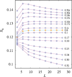
Figure 2. Finite-size results for the scaled magnetic gaps  of the generalized Baxter–Wu model with several values of
  , as indicated at the right-hand side of the figure.
Download figure:
Standard image High-resolution imageFor comparison, we also show similar results for the four-state Potts model on the square lattice. Figure 3 shows the scaled magnetic gaps for two transfer directions, together with part of the results for the generalized Baxter–Wu model. For small L, the difference between the two sets of Potts data display a rapidly decaying L-dependence, indicating the presence of terms with power-law dependence on L. For larger L the dependence becomes rather weak, similar to the generalized Baxter–Wu results. These data suggest that the marginal field in the Potts model with nearest-neighbor interactions on the simple quadratic lattice corresponds to about  in the generalized Baxter–Wu model. Our next task is to check to what extent equation (6) can describe these data. At the largest system size
  and small marginal fields v, one expects that
  is proportional to
  , with a next order contribution as
  due to the v in the denominator. Dividing out
  , the expected linear behavior is reproduced in figure 4(a). For larger marginal fields, higher-order terms become important. The maximum in figure 4(b) indicates that we will require extra terms in addition to the term proportional to
  .
.

Figure 3. Finite-size estimates of the magnetic scaling dimension Xh of the  Potts model on the simple quadratic-lattice, and for the generalized Baxter–Wu model with several values of
  as indicated at the right-hand side of the figure. The red squares show data for the
  Potts model, with transfer directions along a set of edges (upper squares) and along a diagonal direction (lower squares). These data apply to finite sizes (horizontal axis) up to 16 and
  respectively. The data for the generalized Baxter–Wu model are shown as circles, and are obtained using a transfer matrix perpendicular to a set of edges, for system sizes up to
  .
.
Download figure:
Standard image High-resolution image
Figure 4. Dependence of the scaled gap, expressed by the quantity  on the marginal field parametrized by
  . These data apply to a fixed finite size
  in
in  . For small marginal fields (a), one finds almost linear behavior, but on a larger scale (b), nonlinearities become prominent.
Download figure:
Standard image High-resolution image3.2. Fitting the Xh data for the generalized Baxter–Wu model
After obtaining the finite-size data for  , and thus having suppressed the power-law corrections to scaling that still occur in the
  Baxter–Wu model, we applied least-squares fits to the quantity
  , based on equation (6) as follows:

The parameter u, which remains to be determined, fixes the relation in lowest order between the marginal field v and  as
as  .
.
The amplitude of the  logarithmic term in the first sum is independent of
  and should, for relatively small
  , yield the dominant contribution to
  . The amplitude s1 should thus be easily be resolved, without much interference from the second-order term which is proportional to
  , and without much interference from the denominator. Then, the next step is to include larger
  , in the hope that the fit can disentangle the contribution with amplitude s2 from the
  dependence of the denominator of the first logarithmic term, which also behaves as
  for not too large
  .
.
In addition to the unknown parameters in the fit formula, we are also interested in their margin of uncertainty. Since the deviations between numerical data  and
and  as computed from the fit formula are not of a statistical origin, the usual procedure is not applicable. We first define the residual as

which takes into account the data with small  can be fitted very precisely with small contributions to higher-order terms in
  . The additional weight factor
  accounts for the reduced precision of the transfer-matrix results for the largest L. After minimizing R, the scale of the deviations between the actual and computed values of
  follows as
  where n is the number of data points. Next we ask the question what deviations in the fit parameters are still acceptable. For data with errors of a random nature, the answer is provided by standard statistical analysis based on numerical errors in
  of magnitude
  . In the present case this answer does not apply, but it may still serve as an order of magnitude estimate. A more reliable estimate of the margin in the fit parameters is obtained by varying the number of fitted parameters, the range of
  , and the cutoff Lmin at small system sizes.
We included fits with only one logarithmic term, the one with amplitude s1. These yielded only consistent results in a rather narrow range of  , so that the parameters u and s1 could not reliably be determined. Results of various other fits with more than one logarithmic term rather consistently yielded
  , and
, and  . For a few of these fits, the parameters are listed in table 1. We also investigated the effects of a nonlinear term in u proportional to
  . Its influence is very similar to that of adding a next term in the sum on k in equation (16), and we were unable to find a significant result for its amplitude. Since the coefficients bi may depend on the marginal field, we also included a term proportional to
  , but its amplitude is small and did not significantly reduce R.
Table 1. Least-squares fits to the finite-size data for  of the generalized Baxter–Wu model with transfer perpendicular to a set of edges. Estimated uncertainties in the last decimal place are shown between parentheses, 'f'means that the parameter was fixed. These error margins are based on statistical analysis and may, at most, serve as an order-of-magnitude estimate. A better indication of these errors is provided by the differences between the fits. The residual R, defined in the text, is also listed.
| Param | Fit 1 | Fit 2 | Fit 3 |
|---|---|---|---|
| a1 |  (8) (8) |
 (7) (7) |
 (7) (7) |
| a2 |  (4) (4) |
 (3) (3) |
 (3) (3) |
| b1 |  (1) (1) |
 (5) (5) |
 (7) (7) |
| b2 | 9.53 (3) | 10.46 (4) | 14.4 (7) |
| b3 |  (f) (f) |
0 (f) |  (4) (4) |
| s1 |  (3) (3) |
 (4) (4) |
 (1) (1) |
| s2 | 0.934 (5) | 0.892 (4) | 0.931 (4) |
| s3 |  (7) (7) |
 (5) (5) |
 (5) (5) |
| s4 |  (7) (7) |
 (5) (5) |
44.0 (5) |
| s5 |  (70) (70) |
 (19) (19) |
 (25) (25) |
 |
 (1) (1) |
 (1) (1) |
 (7) (7) |
 |
 |
 |
 |
| Lmin | 12 | 15 | 12 |
 |
0.12 | 0.14 | 0.14 |
With the exception of a3 and a5, most parameters seem reasonably well determined, in particular u, s1 and s2 describing the leading logarithmic terms. The third fit covers the widest range of system sizes and  values. It yields a universal ratio
  , in a reasonable agreement with Cardy's exact value [3]
  . Furthermore, these parameters enable the determination of the marginal field. Using the normalization mentioned in section 2, a comparison between equations (6) and (16) shows that
  . With
  [3], the numerical result for the amplitude s1 then determines the marginal field as
  .
.
3.3. Analysis of the Potts model

In analogy with section 3.2, the finite-size data for  were fitted by

The residual R is simply defined as the sum of the squared deviations between the actual and computed values if  . The value of
  increases rapidly when the minimum system size Lmin is decreased below 10. We were unable to find reliable results from fits with all parameters left free. For this reason, we fixed the known amplitude ratio
  , and
, and  ,
,  ,
,  , and
, and  , as found from the amplitudes for the generalized Baxter–Wu model.
While the numerical uncertainties as listed in table 2 depend on the somewhat arbitrary procedure followed here, and may be underestimated, a comparison between a number of different fits still suggests that the value of w is approximately correct. The value also determines the marginal field via  as
as  , with the normalization mentioned in section 2. We note that the value
  , suggested by the data in figure 3, for the generalized Baxter–Wu model that has a marginal field comparable to that of the
  Potts model, corresponds to
  . This is indeed close to the values in table 2.
Table 2. Least-squares fits to the finite-size data for  of the four-state Potts model for two transfer directions. The second column specifies the transfer direction, along a set of edges (e) or diagonals (d). These fits use a small system-size cutoff at
  for the transfer matrix along a set of edges, and at
  for the diagonal transfer matrix. The amplitudes pi are fixed with respect to the parameter w, using the amplitude ratio as found for the Baxter–Wu model. Although w is the only adjustable parameter describing the logarithmic correction in this fit, the residuals per data point, listed as
  , are rather small. The error margins in the last decimal place, shown between parentheses, are based on statistical analysis and may, at most, serve as an order-of-magnitude estimate.
| Param | Transfer | Fit 1 | Fit2 |
|---|---|---|---|
| a1 | e |  (10) (10) |
0.269 (10) |
| a2 | e |  (2) (2) |
3.0 (2) |
| a3 | e |  (3) (3) |
 (3) (3) |
| a1 | d |  (2) (2) |
0.011 (2) |
| a2 | d |  (6) (6) |
1.5 (7) |
| a3 | d |  (5) (5) |
 (6) (6) |
| p1 | — |  (f) (f) |
0.014 27 (f) |
| p2 | — |  (f) (f) |
0.006 46 (f) |
| p3 | — |  (f) (f) |
0.002 91 (f) |
| p4 | — |  (f) (f) |
0.002 12 (f) |
| p5 | — |  (f) (f) |
0.001 95 (f) |
| lmin | — | 10 | 11 |
 |
— |  (10) (10) |
 (10) (10) |
 |
— |  |
 |
4. Numerical analysis of the free energy
4.1. Preliminary result for the generalized Baxter–Wu model
The critical free energy density is exactly known [20] for  as
as  . The geometric factor ζ is included because the free energy per lattice site is not equal to the free energy density. We can thus estimate the conformal anomaly c from the finite-size data
  , from the relation [21–23]

Analysis of the finite-size data for  reproduces the exactly known value
  within a margin of the order of
  . Next we check to what extent equation (5) describes the v dependence of the critical free energy. We attempt to get rid of the bulk free energy at
  , and of the conformal contribution by defining

Since the finite sizes  , 27 are presumably large enough, it is supposedly justified to interpret
  in terms of the asymptotic scaling properties of singular part of the free energy. Since the marginal field
  , one may expect, on the basis of equation (5), that
  behaves as
  . Then, for sufficiently small values of
  ,
,  should be proportional to
  . This is supposed to hold for real as well as complex couplings. In order to check for possible corrections to scaling not included in equation (5), the quantity
  is plotted in figure 5 versus
  . The smallest value of
  is 0.005, yielding points at an unresolved distance to the vertical axis in figure 5.

Figure 5. Plot of the quantity  versus
  . It describes the dependence of the singular part of the free energy of the generalized Baxter–Wu model on the square of the marginal field which relates to
  as
as  . From equation (5) one would expect, as long as v is not too large, a straight line through the origin. The data points for real couplings are shown as red circles, those for complex couplings as blue squares.
Download figure:
Standard image High-resolution imageOne can make the following observations:
- In the limit , the line does not pass through the origin. This can be simply explained by another L-dependent term in the free energy, for instance one proportional to , and thus also proportional to , which contributes a constant to .
- The line in the figure consists of two branches, of which one corresponds to real values of (first-order range, ), and the other to imaginary (continuous transitions, ). The parabolic approach of these branches to the vertical axis indicates the presence of a small L-dependent contribution proportional to v2 in f.
- The two branches display intersections. The curvature leading to the first intersection is in line with the presence of a term with amplitude v in the denominator. The second intersection corresponds to a higher odd power of v.
- The branches display a general upward curvature that indicates the existence of an L-dependent contribution in f with a higher even power of .
- Apart from the above observations, the expected linear dependence on , as predicted by equation (5), is still visible to some extent in this plot for .


These findings provide some useful information for a more detailed analysis of the free energy.
4.2. Preliminary results for the Potts model

Finite-size data were calculated for the free energy of the square-lattice model, using transfer directions along a set of edges as well as along a diagonal. These transfer matrices add layers consisting up to 16 spins. Since L denotes the strip width in units of lattice edges, the data from the diagonal transfer matrix apply to finite sizes up to  . In order to find out what contributions to the free energy occur, in addition to the bulk term
  and the conformal term
  , we define the quantity
  as
as

The data in figure 6 reveal large contributions to  proportional to
  , corresponding to
  terms in
  . Their amplitudes are seen to depend on the orientation of the finite-size direction with respect to the lattice.

Figure 6. Excess critical free energy of the square-lattice  Potts model, shown as the quantity
 ![$g(L) \equiv L^2[\,f(L)-f(\infty)]-\pi/6$](https://content.cld.iop.org/journals/1751-8121/50/32/324001/revision2/aaa7b53ieqn250.gif) versus
versus  . The upper set of data points is obtained using the transfer matrix for transfer parallel to a set of lattice edges, the lower set uses transfer in the diagonal direction. The latter data use a finite size as
  times the strip width in units of face diagonals.
Download figure:
Standard image High-resolution imageThe data do not approach the limit  at
at  linearly, which is in line with the expected existence of a contribution with a logarithmic dependence on L.
4.3. Comparison of the generalized Baxter–Wu and the Potts model
The bulk free energy is, unlike the  Potts model, not known for the generalized Baxter–Wu model. But we can remove it, by taking differences between consecutive finite sizes. To this purpose we define

where  . This eliminates, at the same time, the conformal contribution at the Potts fixed point. Figure 7 show the numerical results for
  for the
  Potts model, and for the generalized Baxter–Wu model with
  , 0.25, 0.28, 0.3 and 0.32. The figures suggest that the magnitude of the correction to f due to the marginal field in the
  Potts model corresponds roughly to
  in the generalized Baxter–Wu model, consistent with the results from the
  analysis.
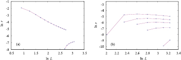
Figure 7. Excess critical free energy of the square-lattice  Potts model, as expressed by the quantity
  , for two transfer directions (a), and for the generalized Baxter–Wu model (b) with
  , 0.25, 0.28, 0.3 and 0.32. Larger
  corresponds to larger
  along the vertical scale. The quantity
  changes sign as a function of L for the Potts model with diagonal transfer, and also for the generalized Baxter–Wu model. The negative entries occur at small L and are left out of these figures.
Download figure:
Standard image High-resolution image4.4. Fit of the generalized Baxter–Wu free energies
First we define

From equation (5), and the observations made in section 4 we expect that

In the numerical analysis, we found that is not well feasible to clearly resolve the logarithmic contributions with amplitudes t3, t4,... when all fit parameters are left free. For this reason we fixed the parameter  as found in section 3 and fitted the amplitudes tk. Since the universal amplitude ratio
  is exactly known [3, 24] we have a consistency check available. The fitting procedure involved the minimization of the residual R defined by
  where yc is computed from equation (24). The roughly estimated accuracies are, in analogy with those in table 1, based on the assumption of randomness. Also for these results one has therefore to estimate the error margins independently by applying several variations of the fitting procedure.
The parameter values as found from two typical fits are listed in table 3.
Table 3. Results of least-squares fits to the quantity  describing the dependence of the generalized Baxter–Wu free energy on
  which parametrizes the marginal field. Errors following from the least-squares criterion are shown between parentheses, 'f'means that the parameter was fixed.
| Param | Fit 1 | Fit 2 |
|---|---|---|
| a1 | 1.307 5574 (2) |  (2) (2) |
| a2 | 0.157 499 (12) |  (9) (9) |
| a3 |  (5) (5) |
 (4) (4) |
| a4 |  (2) (2) |
 (1) (1) |
| a5 |  (2) (2) |
 (1) (1) |
| a6 | 70 (11) |  (3) (3) |
| h1 |  (2) (2) |
 (2) (2) |
| h2 |  (6) (6) |
 (5) (5) |
| h3 | 878 (38) |  (25) (25) |
| t3 |  (2) (2) |
 (16) (16) |
| t4 | 67 (3) |  (2) (2) |
 |
 (f) (f) |
 (f) (f) |
 |
 |
 |
 |
0.2 | 0.22 |
| Lmin | 15 | 15 |
The condition  appears to be approximately satisfied, but there is still an uncertainty margin of the order of ten per cent.
4.5. Fit of the Potts free energy

Taking into account the logarithmic correction term in equation (5), and a few other terms that were found necessary, we fitted the following expression to the data for  defined by equation (21)

where a1 to a3 were allowed to be different for the two transfer directions, while the si and w were taken to be the same. The term with  was suggested by the
  criterion. We do not expect confusion between these si and the sk in equation (16).
Satisfactory fits could be obtained to free-energy data for finite sizes of 8 and more lattice edges or face diagonals. The residual is defined here by ![$R=\sum [g(L)-g_c(L)]/L^2$](https://content.cld.iop.org/journals/1751-8121/50/32/324001/revision2/aaa7b53ieqn303.gif) , where
, where  is the value found from equation (25). The residual is used again to get a rough idea about the numerical error margins in the results for the fitted parameters. These fits were unable to simultaneously determine the parameters w and si, in the sense that the estimated error margins exceeded the actual values. We thus set
  as found in section 3.3. Some typical results for the fitted parameter values are listed in table 4.
Table 4. Results of least-squares fits to the quantity  describing the residual free energy density of the
  Potts model. The second column specifies the transfer direction, along a set of edges (e) or diagonals (d).
| Param | Transfer | Fit1 | Fit 2 |
|---|---|---|---|
| a1 | e |  (2) (2) |
 (2) (2) |
| a2 | e |  (2) (2) |
 (3) (3) |
| a3 | e |  (3) (3) |
 (4) (4) |
| a1 | d |  (2) (2) |
 (2) (2) |
| a2 | d |  (3) (3) |
 (4) (4) |
| a3 | d |  (6) (6) |
 (1) (1) |
| s3 | — |  (2) (2) |
 (2) (2) |
| s4 | — |  (3) (3) |
0.021 59 (3) |
 |
— |  (f) (f) |
 (f) (f) |
 |
— |  |
 |
| Lmin | — | 8 | 9 |
These data lead to a result for the universal ratio  , again close to the exact [3] value
  .
.
5. Discussion
Since the corrections to scaling in  appear in first order of the marginal field v, the data for
  are easier to analyze than those for the free energy, where these corrections appear only in third and higher orders. Moreover, also the analytic background in the free energy depends on
  . But even in the relatively simple case of
  there are complicating factors. There are not only contributions in different orders of the marginal field, but also corrections due to the irrelevant fields of the Potts fixed point. Each of these contributions displays a different L-dependence. The numerical analysis has to separate all these effects, while the range of finite sizes is quite limited. Under these conditions a reasonably accurate and independent determination of the parameters u and s1 in equation (16) was only possible because of the accuracy of the finite-size data for
  , the knowledge of the self-dual points of the generalized Baxter–Wu model, and the fact that in this model the marginal field is continuously variable. Furthermore, the independent determination of u and the si yielded universal amplitude ratios that were used in the analysis of the four-state Potts model, ad thus enabled a determination of its marginal field. It appears that higher-order logarithmic terms in the expansion of
  with amplitudes si and pi are not negligible.
In the analysis of the free energy, we were not able to determine the parameters t3 and u in equation (24) independently, but using the result  from section 3 we could still provide confirmations of the universal amplitude ratio [3]
  .
.
Our numerical work used real×8 floating-point arithmetic and required a computer memory of several tens of Gb. This represents what is reasonably achievable with today's PC's. More accurate results could be obtained in the future by using real×16 floating-point arithmetic instead, which would allow a better separation of contributions in different orders of the marginal field.
Acknowledgments
We gratefully acknowledge the important contributions of Prof John Cardy to the field critical phenomena, which provided key ingredients for much of our work. H B is indebted to Profs Hubert Knops, Hans van Leeuwen, and Bernard Nienhuis for enlightening comments, and acknowledges the hospitality of the Faculty of Physics of the Beijing Normal University. This research is supported by National Natural Science Foundation of China under Grant No. 11175018.