

Abstract
Clean water is key for sustainable development. However, large gaps in monitoring data limit our understanding of global hotspots of poor water quality and their evolution over time. We demonstrate the value added of a data-driven approach (here, random forest) to provide accurate high-frequency estimates of surface water quality worldwide over the period 1992–2010. We assess water quality for six indicators (temperature, dissolved oxygen, pH, salinity, nitrate-nitrite, phosphorus) relevant for the sustainable development goals. The performance of our modeling approach compares well to, or exceeds, the performance of recently published process-based models. The model's outputs indicate that poor water quality is a global problem that impacts low-, middle- and high-income countries but with different pollutants. When countries become richer, water pollution does not disappear but evolves. Water quality exhibited a signif icant change between 1992 and 2010 with a higher percentage of grid cells where water quality shows a statistically significant deterioration (30%) compared to where water quality improved (22%).
Export citation and abstract BibTeX RIS

Original content from this work may be used under the terms of the Creative Commons Attribution 4.0 license. Any further distribution of this work must maintain attribution to the author(s) and the title of the work, journal citation and DOI.
1. Introduction
Water quality deterioration is a global and growing problem for human development and ecosystem health. It negatively impacts health in both the short and long term, and it decreases labor and agri cultural productivity, which may result in lower incomes for people [1, 2]. As a consequence, targets of sustainable development goal (SDG) 6 aim to ensure safely managed drinking water and sanitation services, improve ambient water quality, and protect water-related ecosystems. SDG indicator 6.3.2 tracks bodies of water with 'good' ambient water quality, where 'good' refers to a level of dissolved oxygen, salinity, nutrients (nitrogen and phosphorus) and acidity that does not damage ecosystem and human health. In addition, SDG 6.6 aims at protecting and restoring water-related ecosystems, for which these selected water quality indicators are highly relevant.
Although there are high ambitions in the SDGs to improve water quality, there is a paucity of data across much of the world. Furthermore, when data are available at a given location (primarily in the global north), time series are often incomplete, as illustrated by the GEMStat database (figure 1)—one of the largest databases of in-situ measurements of freshwater quality. In addition, a majority of data points are about 30 years old (figure 1), making them outdated and largely uninformative for policy purposes.

Figure 1. GEMStat data for dissolved oxygen (do), electrical conductivity (ec), nitrate-nitrite (noxn), pH, total phosphorus (tp), and temperature (tw) between 1992 and 2010. The left panel shows the spatial distribution of the original observations per station. Dots size represents the number of observations per station. Dots color represents the number of indicators measured in a station. The right panel shows the temporal availability of data.
Download figure:
Standard image High-resolution imageProcess-based models are currently the main modeling approach to fill data gaps in the water literature. Since 2010, there has been a rapid growth in the number of large-scale models for predicting indicators such as river water temperature [3–6], nutrients [7, 8], organic pollution [9–11], microorganisms [12], chemicals [13], plastics [14], nanomaterials [15] and pesticides. Limited systems knowledge and parameter availability exist to mechanistically predict water quality variations at high temporal and spatial resolutions using process-based models [16]. In other fields, ranging from forest ecology [17] to development economics [18], machine learning models are increasingly used to flexibly predict missing data with high accuracy.
Our paper analyzes the value-added and complementarity of predictive statistics models to traditional process based models in filling global data gaps. We use a fairly standard statistical model, random forests (RFs), to predict six water quality indicators relevant for SDG 6 at a monthly temporal scale between 1992–2010 and globally at a 0.5° resolution. These indicators are dissolved oxygen (do) concentrations, electrical conductivity (ec) for salinity, nitrate-nitrite (noxn) and total phosphorus (tp) concentration for nutrients, pH for acidification and water temperature (tw). We compare our estimates to state-of-the-art process based models [19] to understand the potential of machine learning approaches at large spatial scales. Our modeling efforts complement recent results that have so far focused on nutrient pollution only [20–22].
2. Methods
RFs are an ensemble, nonparametric modeling approach. The approach grows a 'forest' of individual regression trees which improve upon bagging by using the best random set of predictors at each node in each tree.
2.1. Water quality data
We use water quality data from GEMStat which is a globally harmonized database on freshwater quality developed by United Nations Environmental Programme - Global Water Quality (UNEP-GEMS), maintained by the International Centre for Water Resources and Global Change and hosted by the Federal Institute of Hydrology in Koblenz. Raw data for the six water quality indicators are mapped in supplementary information 1. As many observations are not correctly encoded in GEMstat, we clean the raw data to exclude outliers, including observations flagged as 'suspect' by GEMStat. Furthermore, we removed observations with abnormal values regarding the properties of the pollutant (ex: pH > 14, Tw = 0 °C in the tropical band)
6
, and excluded observations that are abnormal regarding the distribution of all observations in a given station and were considered as outliers (i.e. we excluded values xi,t
when in station i,  >[x−
i,t
+ 2.5 σx
], where x−
i,t
represents the average value of all xi,t
in station i at tim t and σx
represents the standard deviations of all xi,t
in station i. The R2 of the final models are not sensitive to the exclusion of these outliers while the root mean square error (RMSE) of predictions decreases. Finally, some countries are overrepresented in our sample (Brazil for DO, TP and Tw; New Zealand for EC; South Africa for NOxN and pH). To limit spatial bias in the results, we randomly sampled observations from the country with the highest number of observations and limit the number of observations to that of the second most represented country.
>[x−
i,t
+ 2.5 σx
], where x−
i,t
represents the average value of all xi,t
in station i at tim t and σx
represents the standard deviations of all xi,t
in station i. The R2 of the final models are not sensitive to the exclusion of these outliers while the root mean square error (RMSE) of predictions decreases. Finally, some countries are overrepresented in our sample (Brazil for DO, TP and Tw; New Zealand for EC; South Africa for NOxN and pH). To limit spatial bias in the results, we randomly sampled observations from the country with the highest number of observations and limit the number of observations to that of the second most represented country.
2.2. Predictors
We constructed a data set of possible drivers to train and predict the model (supplementary information table 1). Data come from 14 sources and include sanitation related variables, gross domestic product (GDP) per capita [23], population [24], urbanization rate, fertilizer use [25], croplands extent, livestock, precipitation and temperature [26], runoff [27], elevation, distance to shore, soil composition (soil pH and EC) [28], and river flows [29]. Squares, cubes, and interactions of variables were constructed to provide additional flexibility to the model. In total, our database contains 66 possible drivers (including squares, cubes and interactive terms).
2.3. Model
Model estimation, fitting, and prediction were done with the ranger and caret libraries in R 4.1 [30–32]. Model training for each water quality indicator was done as follows. First, covariates with a near zero variance were excluded. Second, we randomly split the sample into ten folds and use cross-validation (CV) techniques—meaning that a given observation is used only to train or predict the model, but not for both. Third, we modeled water quality as a function of its drivers. We let the algorithm identify which variables to include for making accurate predictions. We estimate for each water quality indicator 1000 trees. Fourth, we explored which drivers of water quality were selected by the model with variable importance plots. We checked that these drivers are coherent with the literature using partial dependence plots [33]. Fifth, the final model is used to predict global values for all available grid cells (around 60 000), at a monthly time scale between 1992 and 2010. For each pollutant, we statistically analyzed trends in predicted pollution using modified Mann–Kendall trend test to account for auto-correlation [34]. Mann–Kendall tests were performed on a random sample of 3000 grid cells for each pollutant.
We chose RF for its general prediction performance compared to other regression techniques such as linear, partial least squares or support vector regressions. However, RF can present drawbacks, such as its sensitivity to time and/or spatial autocorrelations [35]. Such dependencies may lead to over-optimistic predictions. We test the accuracy of the predictions using station-blocs CV and wa ter basin leave one-out CV (LOOCV). In the station-bloc CV, instead of randomly allocating water quality observations to folds, we attributed monitoring stations to ten different folds and trained the model using CV. In the basin LOOCV all observations from a given basin were successively excluded from the training procedure and only used for testing. This was done to simulate the absence of a large geographical area. Finally, we conducted a temporal validation using an annual LOOCV approach (all observations of a given year are sequentially excluded from the training to be used for testing).
2.4. Area of applicability
The validity and spatial transferability of RF predictions relies on the similarity that exists between the values of the predictors in the training and prediction samples. The spatial imbalances in our training dataset means that our model could not be able to predict trustworthy values for some parts of the world. This is for example the case for Sub-Saharan Africa for which we have extensive observations from South-Africa, and more limited observations from Ghana, Lesotho, Mali, Senegal, Sudan and Tanzania. Recent advances allow us to determine area of applicability (AOA) and dissimilarity index (DI) [36]. AOA is defined as the area, for which the CV error of the model applies. It is based on DI, a metric based on the minimum distance to the training data in the predictor space. We determine the AOA for each water quality indicator [37].
3. Results
3.1. Accuracy
R2 for random splits, basin-block, station-block cross validation, and temporal splits are synthetized in table 1 and illustrated in supplementary information figures 2–5. A high correlation was found between observed and predicted water quality. With standard random splits validation techniques, the model explains 81% of the observed variability in the testing sample for pH, 70% for EC, 79% for DO, 71% for NOxN and 94% for Tw. This performance compares well to, or exceeds, the performance of other recently published process-based models. For example, RMSE of predictions for water temperature is half as large as reported for global process-based water temperature models [3–6]. A lower model performance was found for TP, where it predicts 37% of the observed variability in the testing sample. The prediction power of the models decreases, without collapsing, when using spatially structured CV based on basins or stations. R2 for Tw decreases only from 94% to 87%. For DO and pH, R2 are also preserved, but at lower levels. Higher decreases are observed for EC, NOxN, and TP, particularly for basin-block CV. However, further tests attest that this loss of predictive power is driven by a handful of basins (e.g. Schelbe basin for EC). The model preserves predictive power but cautions need to be taken to interpret local values. When station-block CV is used, more predictive power is maintained compared to basin-block CV. Finally, we follow previous assessments in process-based models by splitting water quality observations into three classes (good, medium or bad, thresholds displayed in supplementary information table 2). Our model accurately predicts the class of water quality and outperforms the process-based models in this task. As an illustration, for salinity, accuracy increases from 80% using a process-based model (appendix B of [19]) to 96% in the data-driven approach described in this paper. Our predictions also compares well to other recently developed machine learning models for nutrient pollutants [21]. The difference in accuracy between the different pollutants is likely to be driven by several factors, including the difference in quality of input data for both the pollutants and drivers, the type of drivers included in the model, and the higher inherent complexity to predict certain type of pollutants than others. This higher difficulty to predict some pollutants more than others, particularly with spatially-structured validation, translates into the number of drivers needed in the model to predict a pollutant accurately (see supplementary figure 7). For Tw, only two drivers have a variable importance larger than 50 (the square and cube of monthly air temperature, supplementary figure 7). On the other hand for nutrient pollutants (NOxN and TP), all 10 drivers included in the model have a variable importance larger than 50 (supplementary figure 7). This highlights the higher complexity to predict nutrient pollution than Tw. For DO, pH, and EC, 2, 5, and 6 drivers have a variable importance larger than 50.
Table 1. Synthesis of models' performance for each type of validation. For random and station cross-validation (CV), ten folds were constructed. For comparability with process-based models such as UNEP [19], we split water quality observations in three classes (bad, medium and good) and determine what percentage of the predicted values for water quality falls into the accurate class.
| Random CV | Station CV | Main Basin LOOCV | Year LOOCV | ||||||||
|---|---|---|---|---|---|---|---|---|---|---|---|
| # Obs. | R2 (%) | Class Acc. (%) | # Stations | R2 (%) | Class Acc.(%) | # Basins | R2 (%) | Class Acc. (%) | R2 (%) | Class Acc. (%) | |
| DO | 81 401 | 79 | 90 | 1724 | 69 | 81 | 173 | 62 | 80 | 90 | 85 |
| EC | 90 993 | 70 | 96 | 1494 | 36 | 87 | 192 | 28 | 86 | 73 | 93 |
| NOxN | 111 535 | 71 | 82 | 2154 | 35 | 57 | 163 | 35 | 43 | 73 | 71 |
| pH | 137 471 | 81 | 98 | 2598 | 64 | 97 | 221 | 41 | 97 | 77 | 98 |
| TP | 78 257 | 37 | 84 | 1610 | 19 | 61 | 135 | 1 | 50 | 38 | 75 |
| Tw | 81 499 | 94 | 96 | 2089 | 9 | 91 | 189 | 87 | 89 | 93 | 93 |
3.2. Predictions
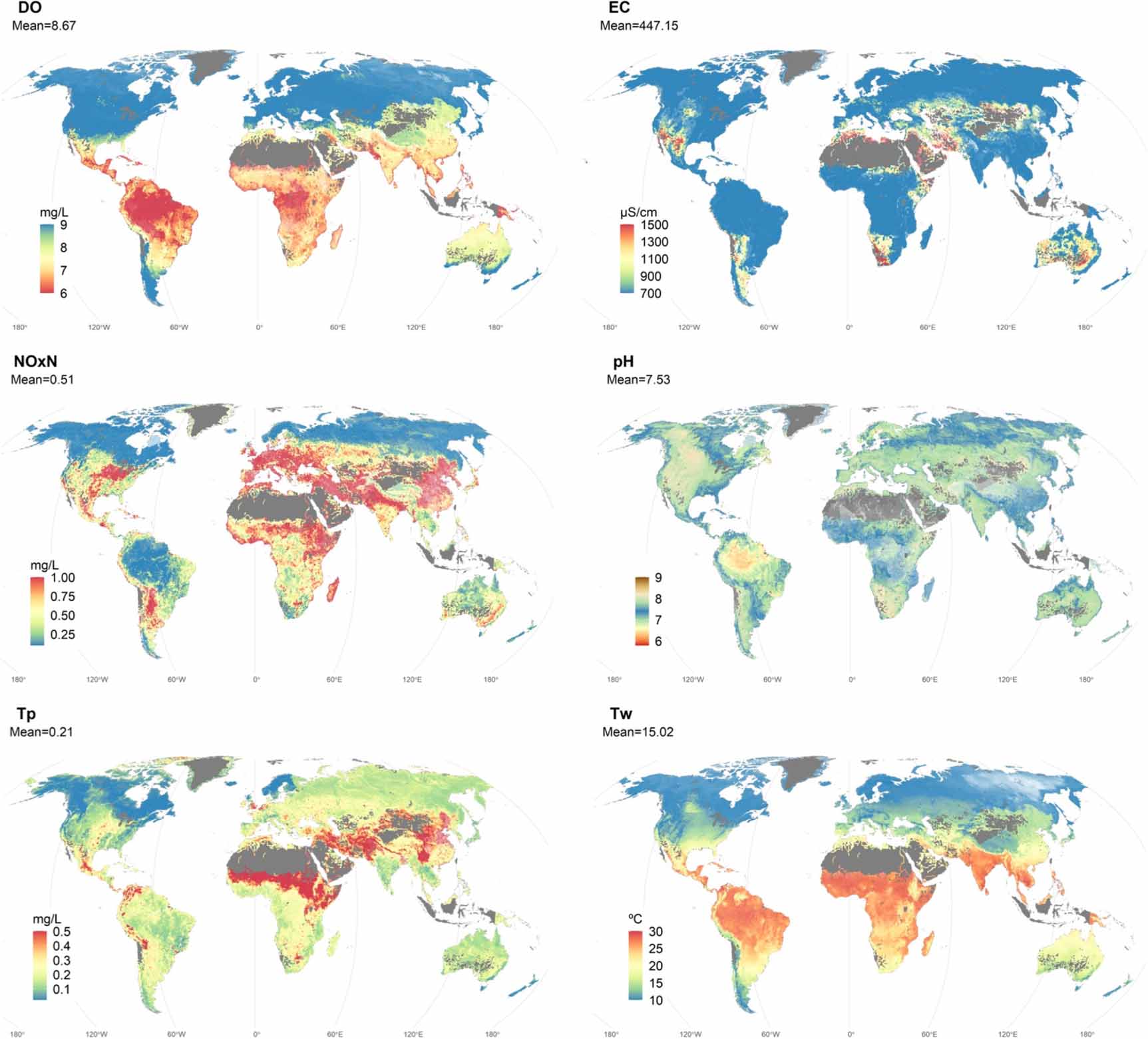
Monthly time series data from 1992 to 2010 are generated for the six water quality indicators. Figure 2 shows the predicted average value of water quality between 2000 and 2010. Figure 3 displays the predicted change in annual average water quality between 1992 and 2010. Table 2 synthetizes the main results of the trend analyses. Water quality exhibited a significant change between 1992 and 2010 in 52% of the grid cells on average. For each pollutant, the percentage of grids where water quality deteriorated (30%) is greater than the percentage of grids where water quality improved (22%).

Figure 2. Global maps of river water quality risks for SDG pollutants dissolved oxygen (DO), electrical conductivity (EC), nitrate-nitrite (NOxN), pH, total phosphorus (TP), and temperature (Tw). Maps below present average values between 2000 and 2010. Regions with river discharge less than 1 m3 s−1 or with missing data on covariates (e.g. Indonesia) are masked (gray). Blue and green represent good water quality, as defined by indicative thresholds provided in supplementary table 2. Yellow, orange and red represent moderate and poor water quality. For Tw, the color coding does not represent quality but the average level. Transparency was added to the cells in which a DI was too high between the training and predictions samples (supplementary information 9).
Download figure:
Standard image High-resolution image
Figure 3. Evolution of water quality between 1992 and 2010 for SDG indicators dissolved oxygen (DO), electrical conductivity (EC), nitrate-nitrite (NOxN), pH, total phosphorus (TP), and temperature (Tw). Values for 1992 were estimated as the annual averages for the years 1992, 93 and 94. Likewise, values for 2010 were estimated as the annual averages of the years 2008, 09 and 10. This was done to limit possible anomalies. Regions with river discharge less than 1 m3 s−1 or with missing data on covariates (e.g. Indonesia) are masked (gray). Blue and green represent an improvement in water quality (e.g. decreases in DO, increases in NOxN). Orange and red represent a worsening of water quality. For pH, deviations with respect to pH = 7 were calculated. For Tw, the water coding highlights cooling or warming. Transparency was added to the cells in which a DI was too high between the training and predictions samples (supplementary information 9).
Download figure:
Standard image High-resolution image
Table 2. For each pollutant, we report the percentage of grid cells showing a statistically significant donward trend, no trend, and statistically significant upward trend between 1992 and 2010 (p-value < 0.05). Trends and significance were tested using modified Mann–Kendall tests to account for serial auto-correlation.
| Pollutant | Decrease (%) | Stable (%) | Increase (%) |
|---|---|---|---|
| DO | 28 | 50 | 22 |
| EC | 25 | 49 | 26 |
| pH | 24 | 47 | 28 |
| NOxN | 26 | 45 | 29 |
| TP | 23 | 43 | 33 |
| Tw | 9 | 55 | 36 |
Supplementary information 7 highlights that a combination of hydro-climatic and socio-economic variables best predict all pollutants. Supplementary information 9 maps DI. The results indicate that for EC, Temp, TP and to a lesser extent pH, we can confidently extrapolate predicted water quality in continents like Sub-Saharan Africa despite the limited input water quality data. This is because the model can complement local African data by data from other continents, possibly at different times (e.g.: Latin America or South Asia in the 1990s shared important similarities with large parts of Sub-Saharan Africa in later decades). For DO and NOxN, the procedure indicates that uncertainties exist in some areas to predict water quality, including in Sub-Saharan Africa.
Unsafe levels of water quality are widely found in most parts of the world, driven by both climate and anthropic pressures. Low-, middle- and high-income countries all face unsafe levels but for different types of pollutants. Our model uncovers water quality hotspots in data scarce regions. Low levels of DO—a sign of unsafe water when levels are below 5–6.5 mg l−1—are widely predicted in large parts of Sub-Saharan Africa, Latin America, and South and Southeast Asia (figure 2). Along with hydro-climatic variables, the lack of access to basic sanitation is a key covariate associated with low levels of DO (supplementary information 7). The infrastructure gap that prevails in most low- and middle- income countries explains these low values of DO. In places where the infrastructure gap has widened because of high population growth and low investment in sanitation, DO has decreased during the study period. This is, for example, the case for coastal parts of China, India, Nepal, or in the northeast region of Brazil.
The concentration of NOxN in water is the highest in densely populated areas with intensive economic activities. England, Belgium, Germany, and some parts of France are the predicted global hotspots of nitrate-nitrite, notably because of intensive animal farming (poultry and pig) and agricultural activities. The challenge of NOxN in most high-income countries has persisted during the period studied and has worsened in fast-growing economies, such as in South Asia, East Asia (e.g. eastern China) and parts of Mexico (figure 3). In these fast-growing areas, intensive animal farming, combined with high population density, excessive fertilizer use, and infrastructure gaps contribute to high nutrient pollution levels (supplementary information 7). A certain degree of caution should be taken when interpreting data from some parts of East Asia, because of the dissimilarities between the training and testing samples for NOxN.
High levels of salinity, as reflected by EC, are driven by geological conditions, drier climates, and the use of fertilizers, which is in correspondence with the overview salinity drivers identified in various river basins across the world [38]. Thus, Australia, Mexico, the Southern USA and Central Asia are salinity hotspots because of their drier climates (supplementary information 7). Over the study period 1992–2010, EC is predicted to have increased the most in India. Turning to Tw and pH, we find that soil composition and air temperature are, respectively, strong determinants of observed levels (supplementary information 6). Large parts of the world have experienced increases in water temperature greater than 1 °C in less than 20 years because of climate variations and change. Such increases in water temperature can have detrimental effects on aquatic life [39–41].
4. Discussion and conclusion
Filling data gaps for water quality will be key to better understanding where hotspots are, to determine trends, and to thus understand our progress towards reaching SDG 6 targets. Data-driven models, based on well-established statistical algorithms, can play a significant role in this endeavor and have shown suitable model performance. They flexibly identifies combinations of factors among a large set of possible drivers to provide accurate estimates of water quality that replicate intra- and inter-annual variations in water quality. They are robust to out of sample geographical predictions and perform at least as well as traditional measurement tools, thus offering a promising path forward for water quality monitoring measurement. Because of their flexibility, high accuracy and ability to model uncertainties, machine learning approaches should be seen as complementary to existing process-based models (e.g. by helping identifying the selection and the inclusion of alternative or additional divers).
Our results show that critical regions and hotspots of water pollution are found across low-, middle- and high-income countries, but for different water quality indicators. Fast growing middle-income countries tend to suffer from a combination of pollutants found in both low- and high-income countries. This is particularly salient when synthetizing all pollutants in a synthetic water quality indicator (supplementary information 10). When the income levels of countries increase, our results illustrate that water quality does not automatically improve: economic development does not solve the problem of poor water quality, but transforms it. In low-income countries, the dominant concern is water pollutants of poverty resulting from poor sanitation and litter that are mostly driven by infrastructure gaps in a fast-changing environment [42, 43]. Elsewhere there are concerns with pollutants of prosperity that result from more intensive economic activities, captured here by NOxN or in other studies by pesticide [44], plastic [14] and pharmaceutical pollutions [45]. Reaching SDG targets will require further investments in treatment, as well as emission control efforts to prevent the pollution from happening in the first place.
Data driven models, such as the one presented here, are an accurate, low-cost and fast method to complement in-situ measurements collected in lakes and rivers. However, the performance of the models also strongly depends on the quality of the input datasets that are used. Although GEMStat is critically important for researchers, policy makers, and civil society, it suffers from important drawbacks. While some regions are well covered in the water quality monitoring database, such as North America, Brazil, and India, other regions such as Central and North Africa, Western and Central Asia, the South Pacific, and Australia are characterized by large data gaps both in time and space. The absence of water quality monitoring data for large geographic areas such as sub-Saharan Africa, might introduce biases in the predictions if there are different drivers of pollution across regions.
Our model serves as a starting point and future work could strengthen the results by expanding to other relevant water quality indicators, using new algorithms (including hydrological grounded models), including more precise drivers, and employing richer water quality training data. We believe that the flexibility of the approach and its transparency can make these machine learning tools useful in the near real-time monitoring of water quality, notably in the context of the SDGs. To this end, an important conclusion of this research is the critical need to expand the spatial coverage of current water quality databases to data-poor regions, notably East-Asia and Sub-Saharan-Africa, to enhance the spatial transferability of the results. This work also highlights importance to sample appropriate anthropogenic and environmental factors that may impact pollution dynamics.
Acknowledgment
For helpful comments and support, we are grateful to the seminar participants at CEE-M, IRD (Espace-Dev), Environmental Justice Programme—Georgetown, the editor and two excellent anonymous reviewers. This paper was part of the 'Quality Unknown' project funded by the World Bank. MvV was financially supported by a VIDI Grant (Project No. VI.Vidi.193.019) of the Netherlands Scientific Organization (NWO). This research was undertaken as part of the Quality Unknown: The Invisible Water Crisis project within the World Bank's Water Global Practice. MvV was financially supported by a VIDI Grant (Project No. VI.Vidi.193.019) of the Netherlands Scientific Organization (NWO).The authors are very grateful for comments from seminar participants at Eco-Publique, CEE-M, Espace-Dev and Georgetown EJP. The findings, interpretations, and conclusions are entirely those of the authors.
Data availability statement
All data analyzed in this study are publicly available. The input data on water quality needs to be requested from GEMSTAT (https://gemstat.org/data/data-portal/custom-data-request/). All data and sources for covariates are presented in supplementary table 1. All predictions, replication data and codes are made available through the platform https://qualityunknown.wbwaterdata.org/.
Authors contribution
S D, R D, J R, E Z, A R conceived the study. S D analyzed the data, with the support of FM, and led the writing of the paper. MvV, R D, J R, E Z and A S R commented on the analysis and provided critical inputs for the writing of the paper. R D led the overall team as part of the 'Quality Unknown' project.
Conflict of interest
The authors declare no competing interest.
Footnotes
- 6
All values outside the following thresholds were systematically dropped: DO ∈ [0, 18 mg l−1], EC ∈ [0, 10 000 µg l−1], NOxN ∈ [0, 90 mg l−1], pH ∈ [0, 14], TP ∈ [0, 90 mg l−1] and Tw ∈ [0, 100 °C].
Supplementary data (6.0 MB DOCX)