

Abstract
Mountains become warmer with elevation in response to greenhouse gas warming, an effect known as elevation-dependent warming. The Eocene is considered a replica of the future climate in an epoch with high atmospheric carbon dioxide concentration (CO2). Therefore, the topographic features of the Eocene strata are of interest. However, obtaining proxy data for mountain regions during the Eocene hothouse is challenging. Paleoclimate model simulation is an effective tool for exploring past climate change. Therefore, we conducted sensitivity experiment simulations employing the Community Earth System Model version 1.2 forced by proxy-estimated CO2 levels. This is the first Eocene study demonstrating the elevation-dependent temperature changes and illustrated using the surface energy budget decomposition. Here five major mountain ranges have been chosen based on their paleogeographic continental location. We found a nonlinear response of elevation-dependent temperature change to CO2 concentrations regulated by seasonal variations. The radiative and non-radiative feedback compensation is responsible for the elevation-dependency temperature changes. Our results suggest temperature perturbations regulate elevation-dependent changes in skin temperature through a combination of feedback under greenhouse warming in the early Eocene. These findings also show future paradox response exhibiting elevation-dependent cooling overall mountain regions due to lower elevation warming.
Export citation and abstract BibTeX RIS

Original content from this work may be used under the terms of the Creative Commons Attribution 4.0 license. Any further distribution of this work must maintain attribution to the author(s) and the title of the work, journal citation and DOI.
1. Introduction
Mountains are an essential component of the climate system; they regulate regional and global climates [1]. Mountain ranges are not only important for the hydrosphere and the atmosphere but also for the biosphere. Due to their altitude, a wide variety of ecosystems and biotopes for rare animals and plants can develop on the slopes of mountains which contribute to the regional biodiversity [2–5]. Although montane and alpine regions are the coolest parts of the land surface, evidence suggests that these regions become warmer monotonously under climate change [1, 6–9]. The majority of high mountains present elevation-dependent warming (EDW) pattern with increased warming with elevation [10, 11]. However, EDW is a regional phenomenon that is not yet fully understood in the context of global warming. Many previous studies have presented well-documented evidence for EDW from observations and modeling for both the present and future in various mountainous regions (e.g. [12–19]). Multiple mechanisms [7, 10] can lead to EDW, and a combination of these mechanisms is responsible for the heterogeneous regional patterns of EDW.
Previous studies have discussed EDW in modern times under climate change using observations, reanalysis, or model output, indicating that various physical processes occurred at different temporospatial scales, potentially providing explanations for the effects of topographic features. These processes were influenced by global warming signals [13, 20]. Often, changes in surface albedo and the related alterations of the net shortwave radiation were listed as the dominant drivers of EDW. However, other processes also contributed to the warming/cooling pattern over complex topography. These include cloud radiative forcing, the effects of changing water vapor contents, the radiative effects of aerosols, and the effects of land cover change [20–22]. In addition to radiative forcing, the heat stored within land surface, ocean surface, or atmospheric circulation can potentially contribute to regional warming [21]. Some studies have pointed out potential mechanisms, such as the latitudinal location of mountain regions or relations to amplified warming in polar regions [12, 21]. On the other hand, some studies suggested an elevation-dependent cooling (EDC), implying more cooling at high elevations compared to low elevations [23, 24]. EDC appeared in response to volcanic eruptions in the last millennium [25]. However, comprehensive studies on the warming climate of past epochs are scarce.
Here, for the first time, we attempted to investigate the sensitivity of the elevation-dependent temperature changes in an early Eocene simulation experiment with varying atmospheric CO2 concentrations. The Eocene was a warm episode in the Earth's history, that occurred approximately ∼56–48 million years (Ma) ago. At that time, atmospheric CO2 concentrations exceeded 1500 parts per million by volume [26]. The Eocene era started with the Paleocene–Eocene thermal maximum (∼56 Ma ago). The global mean surface temperature raised from 5 °C to 9 °C because of the high atmospheric CO2 concentration [27, 28]. This era is considered a replica of future climates owing to the high projected greenhouse gas concentrations [29–31]. Paleoclimatic model simulations [32–34] have thus been used to understand past climate change and its features.
Global climate models (GCMs) offer a tool to replicate possible climate outcomes in future or past, when observations were not available, in response to changing CO2 concentration. Model sensitivity scenarios forced by data of palaeo climate proxies were found to replicate the past climate reasonable well, with lower temperature gradients in the tropical sea surface temperatures being warmer than those in modern times [32, 35–40]. Using such an approach, we can answer some challenging questions, such as how sensitive elevation-dependency on temperature was to increasing CO2 levels in the past? The main objective of the present work is to explore elevation-dependent temperature features in early Eocene simulations under an extreme warming condition using the Community Earth System Model version 1.2 (CESM1.2) [41] model simulation. This allows us to investigate both elevation dependency of various climatic and thermal conditions, regionally and globally, and its sensitivity to a large varying CO2 concentration in the atmosphere.
2. Methods
2.1. Model experiment
To study the elevation-dependent temperature changes during the Eocene hothouse, we investigated CESM1.2 model simulations which is available at the deep-time model intercomparison project framework (DeepMIP, described in [33]). All participating modeling group experiments were forced by proxy-estimated CO2 levels. The model simulation was performed with CO2 concentrations from 280 ppm (pre-industrial levels) to 2520 ppm (9 × CO2). As our ultimate goal was to investigate elevation-dependency on the temperature at various atmospheric CO2 concentrations, we used CESM1.2 simulations for the following reasons. First, its sensitivity experiments operate with atmospheric CO2 concentrations ranging from 1 to 9 times the pre-industrial value, under paleogeography with vegetation type conditions, and river routing [42] and preindustrial levels of other gases and orbital forcing. Second, this model shows an overall agreement with proxy records and captured realistic greenhouse warming features during the early Eocene [40, 43]. Even though proxy-estimated data during Eocene are limited, the model simulated zonal mean temperature over land illustrates consistency among corresponding proxy estimates (supplementary figure 1). CESM1.2 configuration used in this study consists of the Community Atmosphere Model 5.3, the Community Land Model 4.0, the Parallel Ocean Program 2, the River Transport Model, the Los Alamos sea ice model 4 and a component coupler [41].
All CESM Eocene simulations were conducted on the horizontal resolution of 1.9° × 2.5° over the atmosphere and land with 30 hybrid sigma-pressure model levels in the atmosphere. The ocean and sea ice at a nominal 1° grid with 60 vertical model levels in the ocean. All CESM model simulations have been integrated for 2000 model years, except for 1 × CO2, which ran for 2600 model years. To make the model suitable for a paleoclimate simulation under a high CO2 scenario, the model radiation code has been slightly upgraded to represent missing diffusivity angle specifications [40, 44].
In addition to the different CO2 experiments (1 × CO2, 3 × CO2, 6 × CO2, and 9 × CO2), a pre-industrial simulation based on the CMIP5 standard was considered for comparison. The pre-industrial simulation 1 × CO2 attempted to represent the preindustrial climatic conditions and 4 × CO2 were conducted to represent the future conditions. However, DeepMIP simulations starting at CO2 concentration equal to the pre-industrial conditions assumed a planet without a permanent ice sheet or sea ice cover at the poles [45]. Here, we have considered the climatological mean state from the equilibrated last 100 model years of each simulation.
2.2. Land contrast
2.2.1. Land amplification
The land amplification factor was calculated [46] using the ratio of land warming per unit of zonally averaged warming of the adjacent oceans (Globally, longitudes from 0° to 360°),
where ΔTL is the change in local air temperature over masked land (latitude from −90° to 90°), and ΔTo is the zonally averaged change in air temperature over the ocean.
2.2.2. Polar amplification
The polar amplification factor is expressed [47] as ratio of the change in temperature over land to the corresponding change in global mean temperature,
where ΔTgm is the change in the global mean temperature.
2.3. Mountain regions and elevation-dependency of the variable
The model elevation topography was available for each grid resolution used in the model simulation. High mountains were assumed to have an orographic elevation of more than 1 km. Therefore, we screened out orographic regions that exceeded 500 m or more in height (figure 1). For the present analysis, we selected the five major high mountain ranges during the Eocene era, as shown in figure 1(b). The regions were the North American mountain range, the Asian mountain range, the Indian Island mountain, the South African mountain, and the Antarctic mountain range. To derive the elevation dependence of warming, we created vertical profiles using equally sized altitude bins with 500 m intervals. To make a bin, we detected the model elevation at each elevation grid point and clustered them starting from 500 m to the mountain summit and taken average at that mid-class interval (supplementary figure 2). Depending on the size of the respective region and the estimated elevation in the paleogeography, the size and number of bins may vary. The mean temperatures of the grid points in each elevation bin were calculated and changes from the sensitivity experiments relative to the preindustrial simulation are represented by lines in supplementary figure S2. The elevation-dependency of the change in the variables was computed by taking the slope between the variable and elevation over each individual mountain range. Least-squares regression was utilized for calculating the slope.
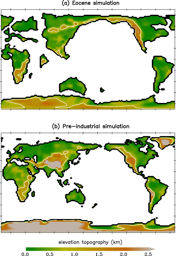
Figure 1. Elevation topography map displaying (a) Eocene simulation and (b) pre-industrial simulation from CESM1.2. White contours represent the global mountain systems (those with elevations higher than 1 km).
Download figure:
Standard image High-resolution image2.4. Surface energy budget decomposition
The surface energy budget analysis used to investigate the causes of elevation-dependent temperature sensitivity can be written in the following form:

where Q denotes land surface heat storage and ground heat fluxes,  is the downwelling shortwave radiation,
  is the downwelling longwave radiation,
  is the longwave radiation from the surface, and (S
+
L) is the turbulent sensible and latent heat fluxes, respectively. Here all fluxes were described as positive (negative) when upward (downward). The equation (3) can be rewritten as:
is the longwave radiation from the surface, and (S
+
L) is the turbulent sensible and latent heat fluxes, respectively. Here all fluxes were described as positive (negative) when upward (downward). The equation (3) can be rewritten as:

where  is the surface albedo considered as a ratio of upwelling to downwelling shortwave radiation for clear-sky conditions.
  can be expressed as
  σTs
4 as a function of the surface radiative/skin temperature Ts, the approximated surface emissivity ( =1), and the Stefan–Boltzmann constant (σ).
σTs
4 as a function of the surface radiative/skin temperature Ts, the approximated surface emissivity ( =1), and the Stefan–Boltzmann constant (σ).
Considering changes in the surface energy budget with respect to changing CO2 concentrations, following the previous methodology [48, 49],
In equation (5),  denotes the change in the high CO2 scenario (3×, 6×, and 9×) with respect to 1 × CO2.
Lu and Cai [48] defined the cloud radiative effect (CRE) as the difference between the all-sky and clear-sky radiations at the surface,

where overbar denotes 1 × CO2 mean state.  and
and  calculated by taking difference between all-sky condition and clear-sky condition radiative fluxes.
Using equation (6), we can rewrite equation (5) and divide it by  will give us the surface skin temperature changes into partial temperature contributions, resulting in the linearly decomposed form as follows:
Each term on the right-hand side of equation (7) contains the partial temperature change due to the corresponding CO2 scenario, which are surface albedo feedback (SAF), the CRE, changes in shortwave radiation for clear-sky not related to SAF (SWCS), longwave radiation for clear-sky (LWCS), land heat storage (HSL), and surface turbulent fluxes (FLUX).
We performed the above calculation at each model grid. Furthermore, we illustrated it in the form of elevation dependency as our study mainly emphasizes elevation-dependent temperature response.
3. Results
3.1. Paleogeography and land warming in the Eocene
A significant difference in the land-sea distribution was evident in the paleogeography [42, 50] compared with a modern topographic map (figure 1). According to the plate tectonics theory [51], continent orientation and ocean bathymetry differ. In the Eocene, mountains were less elevated, and their orographic features were quite different from those in the Anthropocene. Large mountain chains were distributed globally, from the tropics to the poles, and were more concentrated over the mid-latitudes. Figure 1 shows the global mountain ranges in Eocene and pre-industrial simulation. For instance, the highest mountains were located in North America (Rocky Mountains) and the Antarctic during the Eocene, with vegetated land surfaces devoid of a permanent ice sheet [33, 42]. As the Indian subcontinent was not yet connected to Asia, the Tibetan Plateau and Himalayan orogenesis had not occurred. Instead, mountains were distributed on the eastern side of Asia. South Africa had a distinct orography.
The specialty of paleogeography is not just limited to topographic features but also land–sea contracts. Land–sea contrast is a fundamental aspect of the climate system that triggered regional impacts [52, 53]. Figures 2(a) and (b) shows overall land, and polar amplification, respectively, in response to 9 × CO2, the scenario with the highest CO2 concentration in the sensitivity experiment (and more information can be found in supplementary table 1). This indicates that there was more prominent warming over land than compared to the ocean, implying that moistening rate with warming over the ocean was greater than that over land (figure 2(a)). The atmosphere gets moister with the ocean warming as the amplification factor is positive, which is nothing but land warming per unit zonal mean warming of the surrounding oceans. The polar amplification response to 9 × CO2 was also evident with land amplification, with more coverage toward the poles (figure 2(b)). The zonal mean land amplification spread can be seen in the sensitivity experiments. However, the high-elevation warming response (figure 2(e)) was comparatively lower in the context of land amplification, except at the South Pole. This also authenticates that the mean global mountain warming rate is the same in all Paleocene CO2 responses and nearly consistent with future CO2 responses, revealing the importance of elevation topography (supplementary table 1). Therefore, we need to carefully analyze the climate response of mountains on a regional scale. Our primary objective is to explore the elevation-dependent temperature response in the early Eocene and assess its sensitivity to CO2.

Figure 2. Amplification response in the context of the land warming. The upper panel shows the spatial map for (a) land amplification factor response to 9 × CO2 and (b) polar amplification factor response to 9 × CO2; high elevations (<1 km) regions indicated with magenta contour. Panel (c) shows the zonally averaged land amplification factor, (d) shows zonally averaged polar amplification factor, and (e) shows zonally averaged high elevations response to mean global warming (GW). Dashed-line indicates 1 °C temperature response. Note that colored lines in panels (c)–(e) denote Eocene simulations, while the black line shows future simulation based on the preindustrial boundary conditions.
Download figure:
Standard image High-resolution image3.2. Elevation-dependent temperature sensitivity
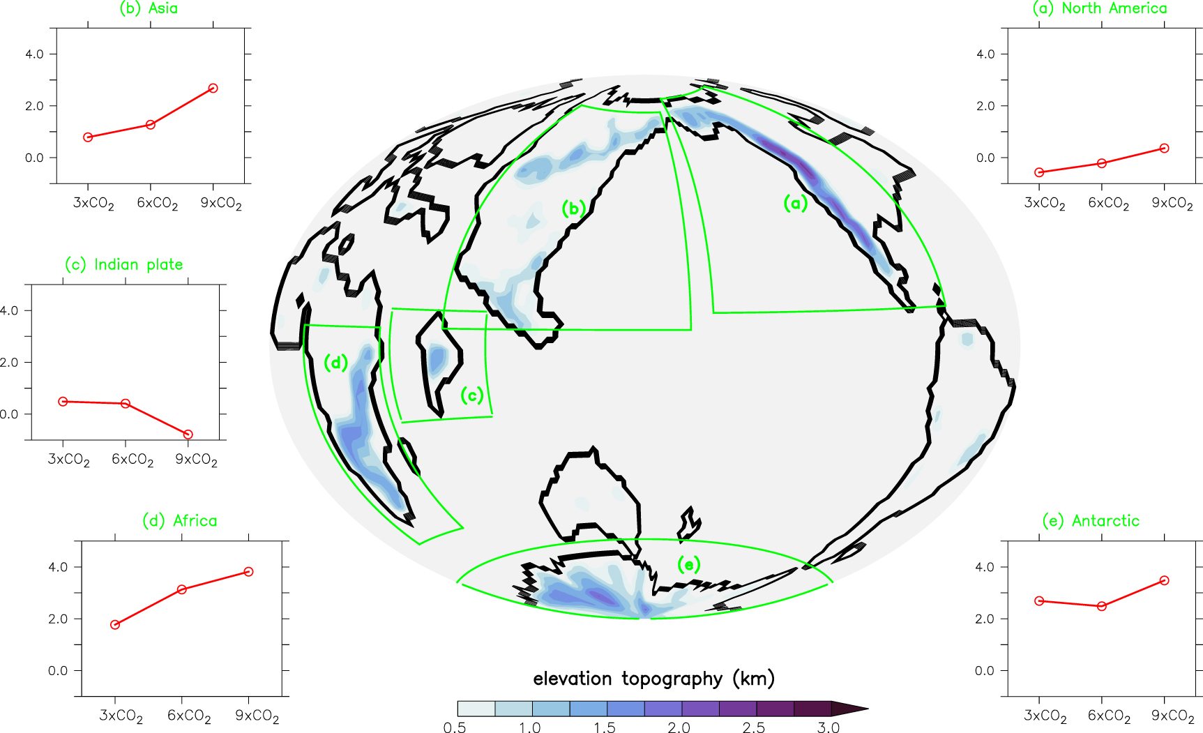
The elevation-dependent temperature change was evident in both hemispheres (figure 3). However, its sensitivity differed across regions and, with CO2 concentrations. Here, the slope estimation method indicated the elevation dependency as a linear function, which may be different from that in the real world. The EDW was explicitly amplified at 3 × CO2 over Asia, Africa, and the Antarctic. The EDW exists over Asia, Africa, and the Antarctic under 3 × CO2, furthermore heightened under 9 × CO2 response. In addition, the chaotic shift from EDW to EDC was observed in the Indian plate (figure 3(c)). In contrast, North America shows both flavors of elevation-dependency with less sensitivity under CO2 concentrations; it shows EDC in 3 × CO2, but an EDW signal emerged with increased CO2. Such mixed behavior of elevation-dependent temperature changes among the mountains underscores the complexities across the globe. These changes range from −0.5 °C to 4 °C km−1, slightly negative to strongly positive across the six mountain regions. Interestingly, this temperature gradient seemed more tilted towards the Southern Hemisphere's response to Antarctic amplification. These elevation-dependent changes in surface temperature showed a nonlinear response with more sensitivity to higher CO2 concentrations.

Figure 3. Eocene mountains representation in CESM1.2 model simulations. Blue shading indicates elevation topography, with an estimated altitude higher than 500 m. The green boxes frame indicates high elevation gridpoints in selected major mountain ranges in this study, including (a) North America, (b) Asia, (c) the Indian plate, (d) Africa, and (e) the Antarctic. Related panels illustrate the regional elevation-dependent temperature (unit °C km−1) under CO2 response realtive to 1 × CO2.
Download figure:
Standard image High-resolution imageFigure 4 depicts elevation-dependent temperature changes using surface air temperature (T) and skin temperature (Ts). Both temperature changes have notable seasonal variations with an almost identical pattern in the elevation-dependent temperature response, pointing to a close connection between them. The monthly variation increased with higher CO2 concentrations over each mountain range, and seasonally the reversed response can be noticed at some places. For instance, North America shows EDC during winter, with small values replicated with the CO2 scenario. However, EDW in summer in higher CO2 scenarios counteracts the EDC resulting in an altogether EDW in North America (figure 4(a)). The mountain ranges in Asia and Africa experienced EDW in all seasons with different intensities and sensitivities to increasing CO2 levels, showing very high values and sensitivity in summer, with opposite trends in winter (figures 4(b) and (d)). Similarly, Antarctica showed the most substantial EDW seasonality. In this region, the EDW was the strongest having its highest peaks in the austral summer (December, January, and February), with especially high sensitivity in January. In the austral winter, values are near zero or showed slight EDC (figure 4(e)). In contrast, the Indian plate experienced a decrease in EDW with increased CO2 concentration (3 × CO2 and 6 × CO2) and EDC (9 × CO2). These effects were reversed in the scenario with the highest CO2 concentration and weak seasonality (figure 4(c)). This seasonal cycle showed the dependency of surface air temperature on the skin temperature CO2 forcing. Surface skin temperatures would not respond similarly to surface air temperatures because of the impact of large-scale circulation [46]. The pattern was almost the same for both temperatures; it was more intense in the case of skin temperature. Surface air temperature may be controlled by large-scale circulation; it usually follows the skin temperature, depending on the turbulent fluxes from the surface. These fluxes play an essential role in air–land surface interactions. The air–land surface temperature change and its interaction can be expressed as an imbalance in the surface energy. The skin temperature over land is strongly coupled with sensible heat flux, which is part of the non-radiative feedback.
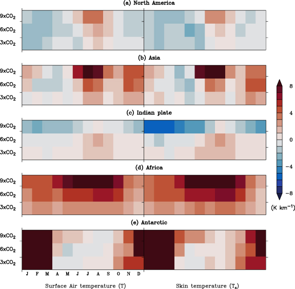
Figure 4. Monthly evaluation (seasonality) of elevation-dependent response of 2 m air temperature and skin temperature to CO2 concentrations for the mountain ranges during Eocene over (a) North America, (b) Asia, (c) the Indian plate, (d) Africa, and (e) the Antarctic.
Download figure:
Standard image High-resolution imageUsing the correlation method, previous studies analyzed the driving mechanisms on the interannual-to-decadal scales [8, 14, 19, 54] However, it cannot be applied to the seasonal scale and is also limited in sense of partial contribution to temperature. A previous study [22] specifically investigated the heat storage term using the surface energy budget for the Tibetan Plateau. This study found increased net radiation at the surface due to a decreased total cloud, and surface snow is favorable for EDW response to 4 × CO2 over the Tibetan Plateau. We attempted to attribute elevation-dependent changes in terms of partial contributions to temperature change and its slope using the model framework.
3.3. Partial contributions from radiative and non-radiative feedback
Figure 5 illustrates the decomposed partial temperature contribution of different terms affecting the energy and heat budget in mountain regions, which can help elucidate the main contributors to the changes in elevation-dependent temperature changes. Such approaches have been extensively used to attribute polar amplification [48, 49]. The terms in equation (7) indicate the partial contributions to CO2-induced warming and consist of radiative and non-radiative feedback processes. Among these terms, SAF, CRE, SWCS and LWCS represent the radiative processes and HSL and FLUX indicate non-radiative processes. Asia, Africa, and Antarctica have EDW signals and a decrease in EDW or even EDC on the Indian plate, while North America owns mixed signals with increasing CO2. However, major contributors differed between mountain ranges due to their geographic locations. The LWCS mainly consists of water vapor and cloud feedback [11, 55, 56]. Meanwhile, the SAF is an important contributor to warming in mid- and high latitudes, although it is negligible in low-latitude mountain ranges. Other contributors counteracted this warming trend, including the CRE, SWCS, and LWCS. However, LWCS can seasonally contribute to enhanced EDW. It implies that the topographic process might be enhanced with CO2 forcing and is consistent with earlier studies [22, 57], which also attributed a similar term [11, 58–60] as LWCS. The CRE was dominant in low-latitude regions, including the Indian plate and Africa (figures 5(c) and (d)). The mountains in South Africa experienced warming mainly because of the LWCS which experienced an increase with increasing CO2 concentration. The EDW followed this trend, while other radiative terms did not show high sensitivity (figure 5(d)). In contrast, in North America and Asia, the SAF contributed to EDW, and changes in LWCS with increasing CO2 concentration enhanced this trend. The SWCS imposed EDC. Furthermore, LWCS and CRE did not present clear signs thus contributing to the seasonality of EDW (figures 5(a) and (b)). Over the Antarctic, which has reduced seasonal ice and snow cover in the sensitivity scenarios (3 × CO2 and 6 × CO2), the strongest EDW was observed with high seasonality. The SAF followed the annual amplitude and season of EDW which is related to snow cover changes. The strong EDW response interpreted in the 9 × CO2 scenario might be due to the polar region's ice/snow cover reduction. A recent study [8, 61] also indicated a current decrease in snow depth over Tibetan Plateau corresponding to EDW. In addition, the LWCS contributed to the warming trend with increasing values with increasing CO2 concentrations (figure 5(e)).

Figure 5. Monthly evaluation of the contribution of partial surface temperature terms to the regional elevation-dependent skin temperature (Ts) change during Eocene over (a) North America, (b) Asia, (c) the Indian plate, (d) Africa, and (e) the Antarctic in response to CO2 concentrations. The term at left axis indicates the elevation-dependent skin temperature change, surface albedo feedback (SAF), the cloud radiative effect (CRE), changes in shortwave radiation for clear-sky conditions not related to SAF (SWCS), longwave radiation for clear-sky conditions (LWCS), land heat storage (HSL), and surface turbulent fluxes (FLUX).
Download figure:
Standard image High-resolution imageThe radiative feedback was strong under CO2 forcing and could explain the EDW pattern and its sensitivity over most of the investigated regions. The results so far describe the radiative feedback effects. Notably, the non-radiative feedback facilitated the radiative contributions and enhanced them. Their negative values (fluxes from land to atmosphere) indicated surface cooling and vice-versa, which ultimately raises the surface air temperature. For instance, the HSL exhibited a similar trend as EDW in North America. The heat stored in the land mass caused the surface temperature to rise, promoting energy release in the form of FLUX (figure 5(a)). The opposite trend can be seen over Africa, where HSL was negative, promoting energy shortage on the surface and triggering positive FLUX values (figure 5(d)). The increased non-radiative feedback (HSL and FLUX), followed by radiative LWCS over the Indian plate under 3 × CO2 and 6 × CO2 scenarios, resulted in EWD from non-radiative processes. However, this could not counterbalance the negative effect of CRE with positive non-radiative feedback, resulting EWC in the 9 × CO2 scenario (figure 5(c)).
The partial contribution of the different terms followed a distinct seasonality similar to that of EDW, which changes with rising CO2 concentration (figures 4 and 5). The total elevation-dependent response and most partial contribution terms to temperature were the strongest in the respective hemisphere's seasonal cycle. Elevation-dependent temperature responses are diverse in each mountains regions with complex local feedback interactions. The SWCS alone did not show this distinct seasonality in any regions and had overall low values. In the summer months, the contribution terms and EDW values were stronger than those in the winter. However, the regions in the Northern Hemisphere did not show seasonality as distinct as those in the Southern Hemisphere. During the summer months in Asia and over the Antarctic CRE and SAF dominated over the radiative terms, respectively, and supported by LWCS, enhanced the seasonal EDW change. The non-radiative terms seemed to counteract these effects (figures 5(b) and (e)). Africa was an exception; here, most terms showed positive values and contributed to warming with elevation. Only slightly negative values were observed for the HSL. The dominant driver for seasonal EDW was LWCS, which was elongated and enhanced by positive CRE (figure 5(d)).
Studies on EDW mainly based on in-situ observation or satellite remote sensing. This is explained by the resolution dependence of micro-physical processes, where resolution dependence of EDW in CESM as thoroughly examined in a previous study using another climate model [19]. Modeling studies supported the assumption, that SAF was relevant in topographic regions where snowline changes [10, 62, 63]. In our paleo-climate setup strongest SAF was indicated for the Antarctic where a melt-down of the entire permanent ice-sheet in the 9 × CO2 scenario would cause an EDW of more than 10 K km−1 in the local winter months. CRE were also handled as major contributors, where temperatures are sufficient high [19]. CRE was most important for the EDC on Indian plate adding about −6 K km−1 cooling trend in the 6 × CO2 and 9 × CO2 scenario, which was not balanced entirely by other processes.
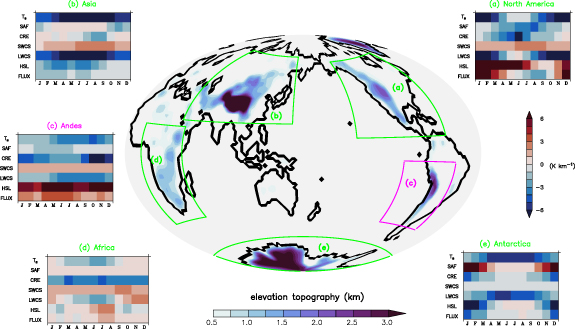
Using present-day-based simulation, all mountain regions (figure 6) reveal EDC in future response to CO2, which is a future paradox. Here chosen regions are slightly different from the Eocene as geography, and continental configuration is distinct in the present day. As the Indian plate is now part of Asia, we consider the Andes mountain range from South America, shown in figure 6(c). These surprising results suggest that future 4 × CO2 responses are in contrast to our Eocene framework and the present agreement, which strongly suggests raising CO2 is responsible for EDW in the future [22, 58, 64]. Even though it is a paradox between the past and the future responses, future EDC is dominantly controlled by LWCS overall mountain regions, underscoring the clear evidence for elevation-dependent water vapor and cloud feedback under future CO2 warming. Numerous studies (e.g. [58, 64]) suggested that LWCS is a potential contributor to EDW; we accomplished this relationship in the past climate during Eocene. Figure 6 shows typical seasonal amplification in radiative feedback and non-radiative feedback. SWCS is the second most dominant feedback after LWCS over North America, Asia, Andes, and Africa. Increasing CO2 in the future can lead to more significant warming at low elevations as we have more elevated mountains compared to the Eocene, resulting in EDC. Many studies also underlined that warming is happening to a certain elevation, supporting our argument. For example, a recent study [20] also infers that the Tibetan Plateau below 5 km exhibit EDW; it did not show any EDW above 5 km or in future climate projections. A study [65] demonstrated Antarctic exhibits low elevation warming in response to 2 ×CO2 forcing. Additionally, this past-future linkage concludes that elevation-dependent temperature changes strongly depend on the geographical orientation of mountains rather than CO2 concentration.
Figure 6. Pre-industrial mountains representation in CESM1.2 model simulations. Blue shading indicates elevation topography, with an estimated altitude higher than 500 m. The green boxes frame indicates elevation gridpoints in selected major mountain ranges for future scenario, including (a) North America, (b) Asia, (c) Andes, (d) Africa, and (e) Antarctica. Related panels illustrate the monthly evaluation of the contribution of partial surface temperature terms to the regional elevation-dependent skin temperature change (unit K km−1) under 4 × CO2 response. The terms are the same as those in the previous figure.
Download figure:
Standard image High-resolution image
4. Summary and conclusions
This present work attempted to explore the past climate response over mountain regions worldwide using a surface energy budget perspective. An analysis based on CESM1.2 showed evident land amplification. In addition, all-mountain ranges experienced elevation-dependent temperature changes during the Eocene in response to CO2 perturbation. Elevation-dependent temperature responses are diverse in each mountain region, with complex local feedback interactions. A nonlinear elevation-dependent response could be observed for selected mountain regions with CO2 concentrations, whereas Asia, Africa, and Antarctica have strong EDW among the mountain ranges. However, North America and Indian plates exhibit mixed signals of EDW and EDC with lower values. We demonstrated that elevation-dependent temperature response was sensitive to seasonal variations. Therefore, this seasonality contributed to the elevation-dependency on temperature and its mean strength.
Here, we use the partial temperature decomposition method to understand physical processes that contribute to elevation-dependent changes. Partial temperature decomposition also suggested that the nonlinear effects resulting from a combination [10] of feedback processes were responsible for the elevation-dependent temperature change over the mountains. The study [22] demonstrated that shortwave radiation is the main contributor to EDW in response to 4 × CO2. However, the present study suggests these interactions are complicated because of their locality, as various terms work differently in elevation-dependent processes. An increase in radiative feedback primarily controlled elevation-dependent temperature change, with the Antarctic exhibiting high sensitivity to CO2. The SAF and LWCS were dominant factors in Antarctic EDW, supported by non-radiative feedback processes. At the same time, the EDC response to 9 × CO2 over the Indian plate occurred despite the negative CRE and SAF supported by HSL. In short, non-radiative feedback supports the radiative adjustment to EDW by enhancing radiative feedback in the early Eocene, and negative non-radiative feedback supported the radiative adjustments to EDW by enhancing radiative feedback. Conversely, a reduction in radiative feedback with positive non-radiative feedback pushes EDC. The equilibrium between radiative and non-radiative processes was responsible for the elevation-dependent temperature changes. We also found a paradox response in present-day based simulation with higher atmospheric CO2 due to the dominant control of LWCS at the lower elevation, resulting in EDC. Previous literature has focused extensively on the EDW in the Tibetan Plateau (the third pole of the earth) in the present and future climate simulations [8–10, 13, 20, 22, 24, 54, 64, 66–68]. However, we found EDC over Tibetan Plateau in response to future CO2, which highlights that elevation-dependent changes strongly depend on the geography of mountains in addition to LWCS. This work also suggests exploring various mountain regions using an energy budget framework can be possible; this can be used to study related elevation-dependent climate change for the past, present, and future.
The regional climate models (RCMs) captures orographic feature better than coarse-resolution GCMs [19, 22, 63, 69]. At the same time, the RCMs has constraints in simulating large-scale features such as global warming. Still, those coarse-resolution GCMs would be valuable in exploring the impact of large scale factors and global warming [11, 19, 22, 64]. The paleoclimate GCMs is usually conducted at a coarser resolution because proxy estimates are limited in numbers and spatial coverage, which also saves computation time. The modeling approach still has some limitations and uncertainty, such as resolution, representation of dynamic vegetation, constant for astronomical parameters, and solar constant. Still, paleoclimate GCMs play a crucial role in understanding paleoclimate features and changes.
Besides, one can resolve the role of polar amplification in global elevation dependency changes for seasonal to interannual scales, which is still an open question for the elevation-dependent climate change research community.
Acknowledgments
The authors would like to express their gratitude to the two anonymous reviewers for their constructive comments and suggestions. This work was supported by the National Research Foundation of Korea (NRF) grant funded by the Korean government (MSIT) (Grant No. 2020R1A2C2006860). The CESM project is supported primarily by the National Science Foundation (NSF). This material is based upon work supported by the National Center for Atmospheric Research, which is a major facility sponsored by the NSF under Cooperative Agreement No. 1852977. Computing and data storage resources, including the Cheyenne supercomputer (10.5065/D6RX99HX), were provided by the Computational and Information Systems Laboratory (CISL) at NCAR. The authors wish to acknowledge use of the PyFerret program for analysis and graphics in this paper. PyFerret (https://ferret.pmel.noaa.gov/Ferret/) is a product of NOAA's Pacific Marine Environmental Laboratory.
Data availability statement
The Eocene simulations used in this study are available by following the instructions at DeepMIP (www.deepmip.org/data-eocene/).
Author contributions statement
P K and K J H conceived this study. P K came up with the initial idea, conducted the investigation, produced figures, and contributed to the initial draft preparation. M B performed data extraction, assisted in the investigation, produced supplementary figures, and contributed to the initial draft preparation. K J H supervised this study, assisted in the investigation, and contributed to writing the draft. J Z performed the model simulations and contributed to writing the draft. All authors interpreted the results and the improvement of the manuscript.