

Abstract
Despite considerable concern about potentially inequitable effects of climate policy, models fall short in assessing their implications for policy design. To address this issue, we develop an agent-based climate-economy model, ABM-IAM, as a disaggregated, behavioural approach to integrated climate assessment. It describes networks of heterogeneous consumers, banks, power plants and firms, and is calibrated on patterns of growth and carbon dioxide emissions generated by the DICE model of Nordhaus. Whereas the latter assumes full employment and abstains from a financial sector and inequality considerations, our approach relaxes these restrictions to obtain a more reliable assessment of climate policy impacts. We show that inequalities in labour and capital income serve as essential but overlooked links between climate-change damages and optimal climate policy. Our result show that lower inequalities of labour income increase the social cost of carbon (SCC), while the impact of capital income inequalities on the SCC depends on the share of population receiving capital rents.
Export citation and abstract BibTeX RIS

Original content from this work may be used under the terms of the Creative Commons Attribution 4.0 license. Any further distribution of this work must maintain attribution to the author(s) and the title of the work, journal citation and DOI.
1. Introduction
The long-term impacts of climate policies have been studied with Integrated Assessment Models (IAMs) that capture the co-dynamics of economy and climate (Tol 1995, Plambeck and Hope 1996, Nordhaus 2016, Weyant 2017). IAMs rely on aggregate equations that describe how accumulation of carbon emissions by production activities affects global temperature, which in turn causes economic damages that reduce economic growth. Here, we take a different approach by proposing a behavioural, agent-based climate-economy model for Disaggregate Climate Assessment. Our model, called agent-based modelling-IAM (ABM-IAM), includes a climate cycle and damages, and describes economic growth as driven by interactions between heterogeneous consumers, firms, power plants and banks interacting within networks. The model is calibrated on patterns of growth and carbon dioxide emissions generated by the well-known DICE (2016) model. We examine how inequalities among households affect the social cost of carbon (SCC). We pay special attention to two mechanisms overlooked so far in the literature: (a) unemployment caused by climate change that increases labour income inequalities; and (b) the impact of capital investments and bankruptcies of firms on capital income inequality. We show that lower inequalities of labour income translate into the larger SCC, whereas the impact of capital income inequalities depends on the share of population receiving capital rents.
The dependence of the optimal carbon tax on inequalities has been studied in three ways: in an intertemporal setting (Anthoff et al 2009, Adler et al 2017); in the context of between-region inequality, with countries being aggregated into a limited number of regions (Nordhaus and Yang 1996, Nordhaus 2017); and focused on within-region inequalities (Dennig et al 2015, Budolfson et al 2017, Kornerk et al 2021). The former addresses inequalities between generations, while ignoring inequalities within them. Governments may respond to the intertemporal inequality by taxing carbon to provide better conditions for the future generations. The disagreement over the value of intertemporal inequality aversion, which measures the concern for the well-being of future generations, has been at the core of the Stern-Nordhaus debate. The second approach is concerned with intragenerational inequity and operates through attaching different weights to regions in the social welfare function used for the climate policy assessment. It has been shown that higher regional inequality aversion increases the SCC (Anthoff and Emmerling 1996).
The third approach examines how the optimal carbon tax is affected by consumption inequalities within-regions (Dennig et al 2015, Budolfson et al 2017, Kornek et al 2021). The study by Denning et al (2015) propose a Nested Inequalities Climate-Economy model that includes sub-regional income quintiles for all of the 12 regions in the Nordhaus's Regional Integrated Climate-Economy (RICE) model 5 . Total consumption in each region is disaggregated into consumption quantiles. Subsequently, the fraction of consumption lost due to climate change in each quantile is computed. The authors compare the consequences of distributing the damage inversely, uniformly and proportionally inversely to income across regions. Regions differ in terms of the total factor productivities. As a result, the way damages are distributed (between regions) affects growth in each region, and subsequently optimal climate policy. The authors show that in case damages fall relatively more on the poor consumers, who are disproportionally represented in the low-income regions, consumption of the poorest regions declines. As a result, the SCC comes out higher compared to other damage distributions.
All three above approaches ignore the impact of inequalities between households on the SCC as their analyses are conducted at a supranational level of aggregation. It has, nevertheless, been suggested that the impact of such inequalities on the SCC may be substantial (Kornek et al 2021). To our knowledge, we present the first agent-based model to study this question. We use the technique of agent-based modelling (ABM) as it is better suitable than representative-agent models to study the distributional impacts of climate change than conventional IAMs or dynamic stochastic general equilibrium models (Farmer et al 2015, Stern 2016, Arthur 2021). Instead of relying on aggregate equations, where consumption of a representative agent is optimized over time, an agent-based model allows us to explicitly describe individual, heterogeneous consumers.
ABMs have been used to study such varied issues as pandemics, bubbles in financial markets, social segregation, diffusion of energy technologies, or job search and matching in labour markets (Windrum and Birchenhall 1998, 2005, Gaffeo et al 2008, Delli Gatti et al 2009, Epstein 2009, Cincotti et al 2010, Neveu 2013, Cardaci and Saraceno 2015, Russo et al 2016, Rengs et al 2020). Macroeconomic agent-based models have been developed as a behavioural alternative to general equilibrium models. Such models have proved capable of explaining core economic phenomena like economic growth, structural change (creative destruction) and business cycles (e.g. Dosi et al 2010). Because of a more realistic representation of agents' heterogeneity, they have opened up opportunities to explore distributional issues (Farmer et al 2015, Arthur 2021). Among others, they have shown that securitization and the emergence of complex financial products can result in a more unequal and financially unstable economy (Cardaci and Saraceno 2015, Russo et al 2016, Botta et al 2021).
ABMs allow for modelling bounded rationality and social interactions, unlike existing climate-economy models which rely on the assumption of representative agents and assume full rationality. Recently, the impact of different types of bounded rationality on the SCC has received some attention in the context of computable general equilibrium (CGE) modelling (Howarth 2006, Gerlagh and Liski 2017, 2018, Chan 2020). However, the ability of such models to study social networks in combination with bounded rationality is limited. While representing an improvement over traditional approaches, such models are unable to fully capture relevant behavioural responses to climate policies, for two reasons. First, behavioural utility functions often complicate analytical solutions or make models so non-linear that an equilibrium may not exist or not be found. As a result, few realistic behaviours have been examined in the context of macroeconomic modelling, despite their relevance for climate policy as indicated by empirical studies. Second, these traditional approaches assume representative agents, thus ignoring diversity of behaviours within a population of heterogeneous agents, such as consisting of consumer classes, as well as preference change due to agents' interactions (network effect). Agent-based models can overcome both these shortcomings.
Only few macroeconomic agent-based models account for the energy sector (Castro et al 2020, Hafner et al 2020). Even fewer account for complex interlinkages between energy, financial sector and climate change (e.g. Gerst et al 2013, Ponta et al 2018, Lamperti et al 2019, Czupryna et al 2020). The study by Lamperti et al (2019) extends the model by Dosi et al (2010) with a climate cycle to examine the public cost of bailout, i.e. rescuing insolvent banks. In their model, climatic shocks reduce the productivity or capital stock of individual firms. Another recent study by Rengs et al (2020) develops a model that includes different classes of households and two types of innovations aimed at improving either the carbon or labour intensity of production. The results show that a supply-oriented subsidy for green innovation can substantially reduce carbon dioxide emissions without causing negative effects on employment.
In this paper, we build upon a previous model that captured complex interactions between the real economy and electricity and financial markets (Safarzynska and van den Bergh 2017a, 2017b). This allows to address multiple inequalities. We extend our model with a carbon cycle consistent with Nordhaus's DICE approach to examine how these inequalities affect the SCC compared with the results of DICE (Nordhaus 2014). The choice of the DICE model is motivated by the fact that it often constitutes the baseline to which other authors compare their results in the literature. Moreover, analytical formulas of the SCC have been derived for the DICE model, which we employ in our model. To our knowledge, we offer the first agent-based model to study distributional impacts of carbon taxes. Existing climate-economy ABMs, such as reported in Lamperti et al (2019) or Gerst et al (2013), do not consider individual consumers but instead assume aggregate demand, which means they cannot address this issue. An exception is Czupryna et al (2020) who consider individual consumers allocating their budget among various goods from distinct sectors. The model describes agricultural, labour and natural disaster damages. However, it has not been used to study climate policies or their distributional consequences.
It is worth noting that the DICE model has been criticized on various grounds (Farmer et al 2015). Especially the dynamics of the climate system have been discussed as inconsistent with the current scientific knowledge. Subsequently, many efforts have been undertaken to improve the model so as to obtain more precise estimates of the SCC (Hansel et al 2020, Dietz et al 2021). We do not intend to contribute to the discussion over the precise value of an optimal carbon tax, but instead want to examine in which direction the SCC will change due to economic inequalities. In the DICE model, total growth and global carbon dioxide emissions determine the value of the SCC. For this reason, we calibrate the model to generate patterns of macroeconomic variables as in the DICE model and examine how introducing different types of inequalities—of capital and labour income and climate damages—influence aggregate patterns.
Our model differs in several respects from the DICE model: for each aggregate equation, we model a network of heterogeneous agents in different markets instead. For instance, capital accumulation follows from decisions of firms who decide whether to expand production. Instead of a single aggregate consumer, we model a population of consumers described by individual heuristics, who spend labour or/and capital income on consumption. Labour income inequalities arise as firms can layout workers if they experience a decline in demand. This way we allow for unemployment, which is absent in the DICE model. The assumption of full employment has been criticized as unrealistic and blurring an accurate assessment of the distributional impacts of climate change (Taylor et al 2016). Capital income inequality depend on the rate of investments in capital by heterogeneous firms. Differential saving rates from capital and labour income have been argued to be a major driver of inequality (Piketty 2014, Milanovic 2016, Ranaldi and Milanovic 2020, Botta et al 2021), but this effect has been ignored in the climate policy assessment. All in all, in our model, labour and capital income inequalities depend on interactions of heterogeneous consumers and firms. The discussed mechanisms are a source of non-linear dynamics, and cannot be studied with highly aggregated models.
The agent-based technique allows us to study systematically how the distribution of climate damages, wealth and capital income among heterogeneous consumers affects optimal climate policy. We find that both wealth and capital income heterogeneity reduce the SCC compared with the egalitarian economy. Capital income allows consumers to smooth their consumption in case climate change pushes them into unemployment, and may mitigate this effect depending on the distribution of capital rents in the economy. In our model, consumers differ with respect to taste: poorer households attach a higher weight to products' cheapness, while richer to their qualities. Either type purchases different goods produced with heterogeneous techniques that differ with respect to labour and energy intensities. As a result, the way how damages are distributed among consumers affects demand for different products, and in turn input use.
Our study relates also to the large literature on the distributional impacts of carbon taxes. The idea is that once the optimal climate policy is determined with highly aggregated models, distributional effects of climate policy can be assessed independently, for instance, using static multi-sector CGE models or micro-simulation models that make the use of microeconomic databases containing data on individual households (e.g. Poterba 1989, Pearson and Smith 1991, Hamilton and Cameron 1994, Metcalf 2008, Rausch et al 2011, Beck et al 2015). For instance, Hallegate and Rozenberg (2017) examine how changes in wages or labour productivities under different climate scenarios affect consumption inequalities, using micro-simulations of 1.4 million households in 92 countries. However, their approach does not account for the policy response to changes in consumption inequalities, as we do. Moreover, existing studies of the distributional impacts of carbon taxes ignore capital income and unemployment effects of climate change. We find that the carbon tax is effective in reducing consumption, income and wealth inequalities over time. The precise effects depend on the relationship between the damage and capital income distributions.
The remainder of the paper is organized as follows. In section 2, we provide an overview of the model. Section 3 summarizes the results from model simulations. Section 4 concludes and discusses policy implications.
2. ABM-IAM
Our model includes heterogeneous consumers, who make decisions on how much to spend on consumption and which products to buy; heterogeneous firms, which offer products that differ with respect to quality as well as price, and compete through reducing costs of production by engaging in innovation activities; and heterogeneous banks and power plants producing energy technologies. supplementary tables ST1-4 summarize all parameters and variables that describe these agents. A full model description is provided in supplementary material 2 (SM2), with its schematic presentation depicted in figure 1. In sections 2.1–2.3, we summarize modifications to a model in Safarzynska and van den Bergh (2017a, 2017b), which we introduce to study multiple dimensions of inequalities and their impacts on climate policies. The model is combined with the climate cycle from the DICE model. The DICE model is also used for the calibration of macroeconomic variables. Altogether, this results in the ABM-IAM model.

Figure 1. Schematic presentation of the model.
Download figure:
Standard image High-resolution imageThe sequence of events in the model is as follows:
- (a)On the market for final products, firms offer products which vary in terms of quality and price. They employ inputs in production and invest in capital expansion; if needed, they ask a bank for a loan to cover costs of inputs. If a new firm tries to enter the market it can receive a start-up loan from a bank.
- (b)Firms set the production level for next period as a weighted average of past sales and production. They set prices to cover the cost of inputs and capital expansion. A mark-up is imposed on the price, which depends on firm's market share. Prices depend also on labour and energy productivities, which change due to R&D investments by individual firms. Firms do not anticipate policy changes, but adapt to them. For instance, a carbon tax increases the price of energy, and thus the probability of firms investing in energy- efficiency improvements.
- (c)Electricity producers generate electricity using distinct energy sources. If an old power plant becomes an obsolete, investments in a new power station are made. The emissions from the electricity sector affect changes in the current stock of atmospheric carbon. Changes in the current stock of carbon affect the global mean temperature above the pre-industrial level, which in turn determine the total damage in the economy, as discussed in section 2.3.
- (d)Total demand for labour in all sectors determines wages in the economy. Consumers receive labour income and a share of capital rents. Consumers decide how much of their wealth and income to spent on consumption in each round. This allows us to examine how differential spending from capital and labour income affects consumption inequalities that are directly linked with emissions.
- (e)Damages are distributed among individual consumers, reducing their budgets according to a parameterized damage distribution function, modified from Dennig et al (2015). We compare three distributions of damages, namely proportional, uniform, and inversely proportional to consumers' wealth (see section 2.2). Differential impact of damages on households can be interpreted as damages affecting labour productivity or causing damage to property of agents, which may vary with households and geographical location.
- (f)Banks pay interest rates on deposits of consumers and firms and collect loan repayments which are due. A bank goes bankrupt if either its equity or its reserves become negative. The model is stock-flow consistent, which implies that all monetary flows are balanced each period. If a bank has no sufficient liquidity to offer loans, it asks other banks at the interbank lending market for a loan. Money supply (M1) is composed of bank money and loans to producers in different sectors.
2.1. Consumption and saving decisions
In the model, consumption-decisions are determined in two steps. In the first step, consumers decide how much of their wealth and income to spent on consumption in the current period. The basic idea is that there is a target wealth-to-permanent-income ratio, which a consumer would like to attain over time (Carroll 2017). The budget determines how many products a consumer can afford to buy in the second step. Consumers' budget  , i.e. how much she spends in time t change according to:
  , where
  and
and  are the shares of income
  and bank deposit
  (i.e. wealth) spent on consumption, respectively. Although shares are the same across consumers, consumers differ with respect to wealth. As a result, more affluent consumers have larger budgets and buy more products. The divergence in the number of products bought by the richest and poorest consumers is weakened by the fact that rich consumers choose better quality and hence more expensive products.
Wealth of each consumer i changes over time: each period, she receives wage (if employed), and in addition a share of energy and capital rents (μsi
). Formally, the deposits of consumer i (Dit) changes according to:  , where rc
is an interest rate paid on deposits;
, where rc
is an interest rate paid on deposits;  is wage; and Cit
is consumption at time t. Parameter μsi
defines the share of energy and capital rents (
is wage; and Cit
is consumption at time t. Parameter μsi
defines the share of energy and capital rents ( ), which a consumer is entitled to. Rents are computed as spendings by firms on inputs, which are not produced in the model, to ensure that the model is stock-flow consistent. For instance, consumption-good firms pay the energy costs to energy firms, but expenses on fuels by the latter constitute dividends. On the other hand, expenses by consumption-good firms on capital (which is not produced in the model) constitute capital rents, which are distributed among consumers.
In the second step, each consumer decides which product to buy by comparing product qualities, prices and adoption rates. In the model, consumers buy products that yield them the highest utility. If such products are out of stock, a consumer chooses probabilistically among available products in the market. The probability  that a consumer buys product j is equal to:
  where uijt
captures utility derived by consumers from purchasing design j, while K captures the strength of market competition. The utility evaluated by consumer i from adopting good j depends on the product quality xjt
, its price pjt
(cheapness), and the number of other consumers who bought the product mjt
:
where uijt
captures utility derived by consumers from purchasing design j, while K captures the strength of market competition. The utility evaluated by consumer i from adopting good j depends on the product quality xjt
, its price pjt
(cheapness), and the number of other consumers who bought the product mjt
:  , where parameter αi
captures i's inclination towards the product quality; α is the network elasticity, where
, where parameter αi
captures i's inclination towards the product quality; α is the network elasticity, where  is firm j's market share. The network elasticity measures the tendency of consumers to follow choices of others. In model simulations, we distribute values of the inclination towards the product quality (
 ) in a way that consumers with more wealth (deposits) at time 0 are assigned a higher value of this parameter. This implies that wealthier individuals are more oriented towards product quality.
2.2. The climate cycle
On the electricity market, three energy technologies compete for adoption: gas, coal and renewable energy. Electricity production by each power plant is described by a Cobb–Douglass function, which accounts for substitution of fuel, labour and capital in electricity generation. Productivities of incumbent plants can change over time due to innovation and learning-by-doing. Output decisions by each plant are modelled as Cournot competition. In particular, power plants decide simultaneously how much electricity to sell on the spot market. If an incumbent plant leaves the market, investments are made in new installed capacity. The decision about the size of and fuel type embodied in a new power plant are based on the discounted value of investments. Each fuel j is characterized by its emission intensity  . The total emissions from the energy sector are equal to:
  , where qijt
is electricity produced by plant i embodying technology j.
, where qijt
is electricity produced by plant i embodying technology j.
The climate module follows Nordhaus's (2017) approach. Changes in the current stock of atmospheric carbon ( ) depend on the existing stock of carbon
  , as well as past emissions:
  , where
  is the permanent stock of carbon (GtC) that stays in the atmosphere for thousands of years;
  is the transient part of the stock (GtC), with Tlag describing how long it takes for the mean global temperature to adjust to an increase in the stock of atmospheric carbon. The permanent stock of carbon changes over time according to:
  , while the transient stock of carbon changes follows:
  . Thus, the current stock of atmospheric carbon depends on a share of carbon emitted into the atmosphere staying there forever (
 ), a share (1−
 ) of emissions exiting the atmosphere immediately, and the part that decays at a geometric rate
  .
.
The stock of carbon  affects the global mean temperature above the pre-industrial level
  according to:
  where
where  is the pre-industrial stock of atmospheric carbon, while
  is the climate sensitivity parameter describing the raise in temperature due to doubling of the carbon stock.
2.3. Climate damages
An increase in the global temperature reduces output according to the damage function (Nordhaus 1994, Nordhaus 2017):  , where
  captures the reductions in total output. Following Dennig et al (2015), we disaggregate total damage among consumers. As consumption is equal to the fraction of output
  , where st
is the saving rate and Yt
total output, both approaches are equivalent in terms of generating the same amount of damage. We refrain from considering damages to capital or labour productivity of individual firms, which has been done elsewhere (e.g. Lamperti et al
2019). This is motivated by the fact that our model excludes catastrophic damages and tipping points (Dietz et al
2021), to make our results comparable with those of the DICE model with gradual damages.
, where st
is the saving rate and Yt
total output, both approaches are equivalent in terms of generating the same amount of damage. We refrain from considering damages to capital or labour productivity of individual firms, which has been done elsewhere (e.g. Lamperti et al
2019). This is motivated by the fact that our model excludes catastrophic damages and tipping points (Dietz et al
2021), to make our results comparable with those of the DICE model with gradual damages.
Formally, damage  is distributed among individual consumers, reducing their budgets by
  , where
  is the share of damages incurred by consumer i. We modify a parameterized damage distribution function based on Dennig et al (2015) by disaggregating damages among individual consumers instead of consumption quantiles as has been done by the authors. The post-damage consumption of individual i (
 ) is equal to:
  , where
  is the number of consumers,
  is the mean consumption, while
  is the share of damages incurred by consumer i. These shares are calculated as follows:
  , where
  is the share of wealth (deposits) hold by individual i at time t;
  is chosen so as to
  . The equation
  captures the relationship between the damage and wealth distributions through assuming a wealth elasticity of damages (ξ). Elasticities of 1, 0, and −1 correspond to damage being proportional, independent, and inversely proportional to wealth. If ξ = 1, the rich are affected the most by climate change, while ξ = −1 implies that damages reduce the budgets of less affluent consumers relatively more. The value of ξ affects only the distribution, and not the total amount of damage.
To illustrate how the distribution of climate damages affects consumers' budgets consider a simple population composed of just two consumers. Of these, one is rich and the other poor: the budget of the rich consumer equals to 8.5, while of the poor 4.5 in the absence of climate change damages. If the economy suffers total damage equal to 5 and ζ = 1, the budget of the rich is reduced to 4.75, while of the poor to 3.35. If instead ζ = −1, the rich consumer can spend 7.25 on consumption, while the poor one suffers disproportionally large reduction in her budget, which becomes 0.75, which would result in larger consumption inequalities. These effects are static. In the model, many differentiated products compete for adoption by heterogeneous consumers. We examine long-term effects using model simulations.
In the baseline model, to which we will refer as the model with rational consumers, we assume no network effect in consumption, while we allow for unemployment. We relax these assumptions in scenarios 4 and 5 described below. In addition, we examine the impact of heterogeneous wealth and rents on the SCC in the following scenarios:
Scenario 1: Just economy
In our model simulations, the wealth of consumers changes over time: each period, consumers receive a wage (if employed), interest on deposits, and a share of capital rents (μsi
). In the 'just economy' scenario, all consumers acquire an equal share of rents, captured through  , where
  is the number of consumers. We further assume that all consumers have the same wealth initially
6
.
is the number of consumers. We further assume that all consumers have the same wealth initially
6
.
Scenario 2: Half-just economy
In 'half-just' economy, all consumers acquire an equal share of rents  —just as in the 'just' economy. However, we assume wealth heterogeneity in this scenario. In particular, in the initial round, we distribute the total wealth W in the economy as deposits among consumers according to the gamma distribution with mean μg.
(⩾1).
—just as in the 'just' economy. However, we assume wealth heterogeneity in this scenario. In particular, in the initial round, we distribute the total wealth W in the economy as deposits among consumers according to the gamma distribution with mean μg.
(⩾1).
Scenario 3: Unjust economy
The 'unjust' economy represents a more realistic scenario, namely with an unequal distribution of rents and wealth, where rents concentrate in a small fraction (10%) of the consumer population. This is motivated by evidence from the U.S., where the top 10% of households own 81% of the total value of those investments (Wolff 2014). A recent analysis indicates that the share of world individuals with positive capital income rose from 20% to 32% between 2000 and 2014 (Ranaldi 2021). We assume rents to be distributed among consumers according to an exponential distribution (see figure 3 in SM2). The distribution of wealth in the first round of model simulations is identical to Scenario 2.
Scenario 4: Full employment
The DICE model relies on the assumption of full employment. Instead, in our model, in each time period, firms revise their demand for labour. We assume a random allocation of workers to firms. Wages are paid only to  workers at time t, where
  are workers employed by a firm j. The total population is constant and equal to
  . In case of excess demand for labour (
 ),
),  of workers remains unemployed, while others receive
  , which can be interpreted as a minimum wage. In case of excess demand, the wage increases over time and it is equal to:
  , thus it depends on the demand and supply for labour. For the purpose of comparison with the DICE model, we conduct additional simulations, referred to as the 'full employment' scenario, where regardless of whether supply or demand is in excess, all workers receive wage equal to:
  . This means that in case
  , the wage is lower than
  , while it is higher otherwise. In both 'full employment' and 'unemployment' scenarios, total spending on labour income is the same, but scenarios differ in terms of labour income distribution.
Scenario 5: Network effect
In the baseline model simulations, we assume that agents are rational by setting the network elasticity to 0. We consider an alternative scenario with boundedly-rational agents, where the network elasticity, i.e. the weight attached to products chosen by the others, is strong (α = 0.15). Both types of agents, i.e. boundedly- and fully-rational, spend the same fraction of income and wealth on consumption.
Scenario 6: A low-growth scenario
The baseline model was calibrated to replicate patterns of macroeconomic variables between 2010 and 2100 as in the DICE (2016) model (section 3). This includes a growth of consumption equal to 1.9%. We introduce an additional scenario, to which we will refer as a low-growth scenario, where the consumption growth between 2010 and 2100 is equal to 1.6%. This is achieved by setting the annual increase in total factor productivity (TFP) equal to 0.01 7 . This scenario is motivated by the fact that current times of high resource costs and economic instability, including due to the invasion of Ukraine by Russia, may affect long-run growth projections downwards.
Scenario 7: The social cost of carbon
We are interested in how equity considerations affect the optimal carbon tax. To this end, we compare the results from the business-as-usual (BAU) scenario in the absence of climate policies with the Optimal Scenario (OPT), where the SCC is translated into a carbon tax on electricity. The SCC measures the net present value of future economic costs arising from an additional ton of carbon dioxide emissions, accounting for the entire path of causes and effects between climate cycle and economic damages (Nordhaus 2017). We use a tax formula proposed by Rezai and van der Ploeg (2016), which is a simplification of one proposed by Golosov et al (2014):  Here γ is a constant scale parameter and ρ a parameter capturing time impatience (set to 0.01, following Rezai and van der Ploeg
8
). We employ this specific formula as it has been derived for the climate cycle consistent with the DICE model. Accordingly, the optimal carbon tax is proportional to the total output. The tax revenue is distributed back to the citizens as a lump-sum equal to all citizens. The resulting tax is optimal by approximation as agent-based models do not allow performing an optimization of output since they involve stochastic elements related to innovations and agent interactions.
Here γ is a constant scale parameter and ρ a parameter capturing time impatience (set to 0.01, following Rezai and van der Ploeg
8
). We employ this specific formula as it has been derived for the climate cycle consistent with the DICE model. Accordingly, the optimal carbon tax is proportional to the total output. The tax revenue is distributed back to the citizens as a lump-sum equal to all citizens. The resulting tax is optimal by approximation as agent-based models do not allow performing an optimization of output since they involve stochastic elements related to innovations and agent interactions.
Scenario 8: Renewable energy
Next, we study the impact of investments in renewable energy on multiple inequalities. In the baseline model simulations, an energy owner invests in a new power station when an old plant becomes obsolete. The size and the type of a new power plant are chosen based on the highest discounted value of such investments. As a result, combined cycle gas turbines (CCGTs) power stations dominate the electricity market as they are the cheapest to install. In the 'renewables' scenario, we assume that whenever a power plant becomes obsolete, an owner of energy plants decides to invest in a new renewable power plant, instead of CCGT, with a probability prenewable equal to 0.5. This may be interpreted as a policy scenario, where the share of renewable energy in electricity production increases over time until reaching on average 50% of electricity production. We consider investments in renewable energy in the presence (OPT) and absence (BAU) of the carbon tax. If the share of renewable energy in electricity production reaches 100%, the tax becomes 0 in the OPT scenario.
3. Calibration and results
We perform simulations with many heterogeneous agents, using the ABM approach. In the supplementary materials, we provide some additional analysis from model simulations, where we doubled the number of consumers, to show that our results are robust to the number of agents 9 . We study model dynamics between 2015 and 2175. Each period corresponds to one year. For each parameter setting, we report mean values over 100 simulations from Monte Carlo exercises conducted with different seeds, motivated by the presence of stochastic factors in our model. Means are calculated over the last 50 years, when model dynamics stabilize, and are summarized in supplementary tables (ST1-ST6).
We calibrate parameters so that the model under full employment in the 'just economy' scenario replicates the aggregate patterns of output and consumption, the carbon cycle, temperature and damages consistent with the DICE 2016 model between 2015 and 2100. Hence, associated parameter values are taken directly from the DICE model, and are described in the supplementary table ST5. The value of the scaling parameter  in the SCC comes from Golosov et al (2014). Other crucial parameters are emissions factors of different energy technologies. We set these so that, consistently with the RCP 8.5 scenario, a temperature increase above the pre-industrial level is between 4 °C and 4.5 °C, while cumulative carbon emissions between 1450 and 800 GtC in 2100, which corresponds to the medium-high IPCC scenario.
Nordhaus calibrates his model, notably TFP, to generate a growth rate of consumption per capita equal to 1.9%. We achieve the same growth rate by setting the increase in TFP equal to 0.05. Other key parameters determining consumption and output dynamics are: the productivity of firms in the manufacturing sector A at t = 0; the share of wealth spend on consumption  and interest rates paid on consumer deposits rc. These are set to 2.5, 2% and 0.1%, respectively. These values are motivated as follows: the initial TFP was set to 2.5 for total output in 2015 to be equal to 75 trillion $. Overall output increases to 300 trillion $ in 2100, which corresponds to the SSP3 projection (Leimbach et al
2017). The marginal propensity to consume out of wealth affects the level of total consumption as well as its growth. The larger the value of this parameter is, the higher total consumption, production and carbon dioxide emissions are. Its value was chosen so that the growth of consumption between 2010 and 2100 is 1.9%. The interest rate on household deposits is set equal to 0.1%, motivated by the range 0.1%–0.14% reported in the U.S. for the period 2011–2015. Other parameter values are taken from Safarzynska and van den Bergh (2017a). We recalibrated some parameters compared to the previous version of the model so that simulations generate dynamics of aggregate variables consistent with the DICE model.
and interest rates paid on consumer deposits rc. These are set to 2.5, 2% and 0.1%, respectively. These values are motivated as follows: the initial TFP was set to 2.5 for total output in 2015 to be equal to 75 trillion $. Overall output increases to 300 trillion $ in 2100, which corresponds to the SSP3 projection (Leimbach et al
2017). The marginal propensity to consume out of wealth affects the level of total consumption as well as its growth. The larger the value of this parameter is, the higher total consumption, production and carbon dioxide emissions are. Its value was chosen so that the growth of consumption between 2010 and 2100 is 1.9%. The interest rate on household deposits is set equal to 0.1%, motivated by the range 0.1%–0.14% reported in the U.S. for the period 2011–2015. Other parameter values are taken from Safarzynska and van den Bergh (2017a). We recalibrated some parameters compared to the previous version of the model so that simulations generate dynamics of aggregate variables consistent with the DICE model.
Figure 2 compares dynamics of income, consumption and wealth inequalities in 'just', 'half-just' and 'unjust' economies under different damage distributions. Income and consumption inequalities are measured through Theil indices, whereas wealth inequality is calculated as the share of total wealth by the richest decile of consumers (top 10%). Patterns depicted in the figure show that climate change increases consumption inequalities in all considered scenarios with no climate change.
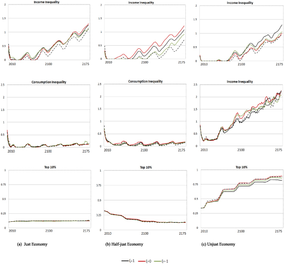
Figure 2. Dynamics of income, consumption and wealth inequalities (top 10%) in the BAU scenario of the model with rational consumers.
Download figure:
Standard image High-resolution imageIn the 'unjust' economy, the trends of all types of inequalities are upward sloping in line with evidence that inequalities are increasing worldwide (Cingano 2014). In turn, in the 'half-just' economy, wealth inequalities are reduced over time. Several studies find that increases in income inequality and consumption are connected (Krueger and Perri 2006, Aguiar and Bils 2015). In addition, evidence indicates wealth and income inequalities are positively correlated, as labour income is a major source of wealth (Berman et al 2016). Wealth inequality exceeds labour income inequality due to rents, dividends or royalties (Piketty 2014). Our model simulations under unequal distribution of wealth and rents replicates these facts.
The upwards sloping trends of inequalities in the 'unjust' economy can be explained by climate damages undermining the purchasing power of consumers, reducing firms' profits and employment. This increases income inequalities, and subsequently consumption inequalities. In the 'just' and 'half-just' economies, consumption inequalities increase less than income. Here, consumers smooth their expenditures with wealth. In the 'unjust' economy, the possibility of smoothing consumption is limited as most consumers do not acquire rents.
3.1. The impact of multiple inequalities on the social cost of carbon
Figure 3 summarizes the main results from our modelling exercises. Figure 3(a) compares the SCC in the baseline model with unemployment to the model with full employment in simulations with rational agents. Figure 3(b) does the same for the models with rational and boundedly rational agents, in simulations that allow for unemployment. We examine if differences in the SCC between distinct damages, wealth and rents distributions are statistically-significant. We do this by running non-parametric tests (the Mann–Whitney tests) on the sample of data consisting of results from 100 simulations for each initial condition (parameter setting). The results are summarized in the supplementary tables 7–12.
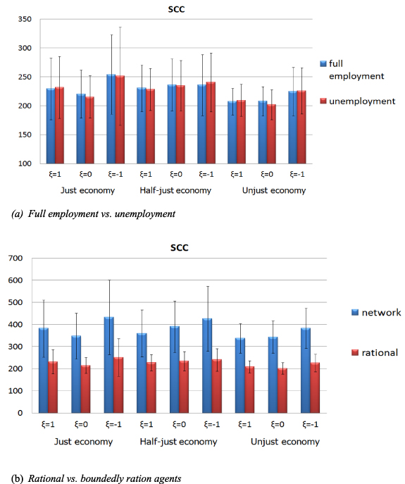
Figure 3. The social cost of carbon under distinct conditions.
Download figure:
Standard image High-resolution imageEvidence in supplementary tables 7(a)–(c) indicates that differences between models with 'full employment' and 'unemployment' are insignificant, regardless of the damage distribution. However, supplementary table 11(c) indicates that differences in the SCC between models with 'full employment' and 'unemployment' are statistically significant for each damage distribution under the low-growth scenario. Here, unemployment reduces the SCC in the 'unjust' economy (supplementary tables 5(c) and 6(c)) 10 . The negative impact of income inequalities on the SCC is driven by the difference in tastes among households. In particular, poorer household buy goods produced with more efficient techniques. As a result, if everyone receives incomes, output growth is higher, and thus emissions and the SCC, compared to the situation where unemployment pushes the least affluent households into poverty, reducing their demand. Another mechanism, which explains our results, is that richer households buy more expensive products that are often characterised by high mark-ups. These have been suggested to be an important driver of labour income inequality, as they decrease the labour share of income (Autor et al 2020). The discussed mechanisms have a stronger impact on the SCC, the lower economic growth is, as this pushes a larger share of the population into poverty.
The main findings from the analysis of our model with unemployment can be summarized as follows (figure 3(b)). First, the SCC is lower in the 'unjust' economy compared to the 'half-unjust economy' scenario. The difference in the SCC between both scenarios is statistically significant for each damage distribution (supplementary table 10(b)). The mean results from Monte Carlo exercises indicate that the tax drops from on average 234.7 $/ton in the 'just' economy to 212.6 $/ton of carbon in the 'unequal' economy. On the other hand, most differences in the SCC between 'just' and 'half-unjust' economies are insignificant (supplementary table 10(a)), indicating that rent inequality has a greater impact on estimates of the SCC than initial wealth heterogeneity.
Second, in the 'unjust' economy, the SCC is significantly larger, when the poor are hurt the most by climate damages (ξ = −1), compared to other damage distributions (ξ= 0 and ξ = 1) (supplementary tables 2(a)–(c) and 8(c)). This can be explained by the fact that over time unemployment unfolds, pushing less affluent households (with low or no savings) into poverty, making them unable to purchase consumer products. As a result, the demand by the poorest households in the 'unjust' economy cannot be reduced further by climate change. On the contrary, climate change reducing budgets of affluent consumers has always a large impact on the total demand, reducing growth and the SCC. In the 'just' and 'half-just' economies, we observe a similar pattern: the SCC is lower for ξ = 1, followed by ξ = 0, and then ξ = −1. However, the difference in the SCC between different damages distributions are not all statistically significant in these scenarios as households smooth their consumption with wealth (tables 8(a) and (b)).
Third, for all considered scenarios, the SCC is greater in the presence of the network effect compared to simulations with rational agents. The differences in SCCs are statistically significant for all damage distributions between scenarios with rational- and boundedly-rational agents (supplementary tables 9(a)and (b)). This can be explained by the fact that rational agents switch to new products easier than boundedly-rational agents. This results in greater market competition (lower H-index of market concentration) and the lower rate of firms' bankruptcies in the model with rational consumers (see supplementary tables 2(a)–(c) and 3(a)–(c)). As a result, new products, produced with more efficient techniques diffuse on the market, which results in lower emissions, and thus the carbon tax compared to the economy with boundedly-rational consumers.
3.2. The impact of the SCC on multiple inequalities
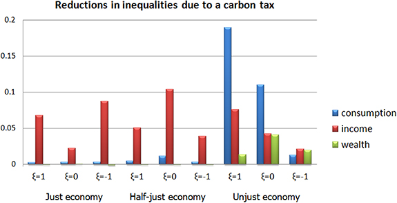
Figure 4 summarizes the reduction in consumption, income and wealth inequalities in simulations with rational consumers. We find that the SCC is successful in reducing all types of inequalities in the long run regardless of the distribution of capital income, wealth or damages. In the model, firms decide whether to invest in improvements in labour or energy productivities depending on the relative prices of both inputs. As a result, the tax induces substitution of energy for labour, while it shifts R&D activities of firms towards improvements of energy productivities. Overall, the tax reduces unemployment, which unfolds over time due to climate change reducing consumers' budgets. The tax reduces also wealth inequalities. These reductions are in general larger in the 'unjust' economy as here the potential for them is greater. Here, the tax is more successful in reducing income and consumption inequalities, the larger the share of damages fall on the rich.
Figure 4. Reduction in income, consumption and wealth inequalities due to a carbon tax.
Download figure:
Standard image High-resolution image
Table 1 presents the results from linear regressions of the logarithm of the SCC on the inequality indicators generated by the model simulations. Each observation comes from a single simulation run of the model with rational consumers. For every parameter setting, we include 100 observations. In the regressions, we pool data from model simulations from three scenarios: 'just', 'half-just' and 'unjust' economy, each run for three damage distributions, which results in total in 900 observations. As an explanatory variable we include consumption, income and wealth inequalities; as well dummies corresponding to different scenarios: 'half-just' and 'unjust' economies. In Model 3, we add interactions terms between different types of inequalities and such dummies.
Table 1. Regressing the impact of multiple inequalities on the SCC (in logarithm).
| Variable | Model 1 | Model 2 | Model 3 |
|---|---|---|---|
| Consumption Inequalities | 0.02 | 0.03* | 0.11 |
| (0.02) | (0.1) | (0.1) | |
| Wealth Inequalities | −0.07 | 0.54** | 0.9 |
| (0.05) | (0.26) | (1.7) | |
| Income Inequalities | −0.81*** | −0.80*** | −0.89*** |
| (0.01) | (0.01) | (0.02) | |
| Unjust Economy | −0.45** | −2.47*** | |
| (0.20) | (0.39) | ||
| Half-unjust Economy | −0.0.003 | −0.56 | |
| (0.56) | (0.34) | ||
| Interaction Consumption Inequality and Unjust Economy | −0.13 | ||
| (0.1) | |||
| Interaction Income Inequality and Unjust Economy | 0.39*** | ||
| (0.04) | |||
| Interaction Wealth Inequality and Unjust Economy | 1.79 | ||
| (1.73) | |||
| Interaction Consumption Inequality and Half-just economy | 0.51** | ||
| (0.10) | |||
| Interaction Income Inequality and Half-just economy | 0.08** | ||
| (0.03) | |||
| Interaction Wealth Inequality and Half-just economy | 3.2 | ||
| (2.7) | |||
| Constant | 6.23*** (0.01) | 6.15***(0.04) | 6.18*** (0.22) |
| No. obs. | 900 | 900 | 900 |
| R-squared | 0.85 | 0.87 | 0.87 |
Note: Standard errors in brackets; ***indicate significance at 1% level; **at 5% level and *at 10% level.
The results in table 1 support that the 'unjust' economy results in the lower SCC compared to the 'just' economy. In favour of this, the dummy corresponding to the 'unjust' economy is positive and significant in Models 2 and 3. Other results indicate that larger income inequalities translate into lower values of the SCC. The variable income inequalities has a statistically significant impact on the logarithm of the SCC in all models reported in the table. This is because labour income is the most important driver of consumption, and thus of production. As a result, higher employment boosts growth, emissions, and the SCC. The impact of income inequalities on the SCC is lower in the 'half-just' and 'just' economies compared to the 'unjust' economy, as indicated by positive and significant signs of the interaction terms between income inequality and the corresponding dummy variables. The higher concentration of capital rents among the smaller share of population is expected to reduce growth, and the SCC. However, wealth inequality turned out to have a negative, yet insignificant, impact on the SCC only in Model 1, i.e. in the absence of scenario dummies.
3.3. Effectiveness and equity of using carbon-tax revenues for renewable energy
Investments in renewable energy are successful in preventing the global temperature from increasing above 3.2 °C by 2100 in the OPT scenario for all damage and capital income distributions (tables 3(a), (b) and 4(a), (b)). In all model simulations, investments in renewable energy reduce (labour) income inequalities. In particular, large investments in power plants act as a demand stimulus, increasing employment (Vad Mathiesen et al 2011). However, in the unjust' economy, investments in renewable energy simultaneously increase wealth inequality. This is because rents from energy and capital benefit disproportionally a small group of consumers. This leads to an increase in consumption inequalities (supplementary tables 4(a) and (b)). Rapid investments in renewable energy come at the cost of systemic risk (Safarzynska and van den Bergh 2017b, Campiglio et al 2018, Semieniuk et al 2020), due to the construction of renewable power plants being more expensive than that of fossil fuel plants. Typically, a single bank cannot afford to finance investments in renewable energy alone and hence borrows money at the interbank lending market. This creates a risk of a cascade of failures in the financial system if a renewable power plant goes bankrupt. Following Tedeschi et al (2012), we measure financial stability by the number of bank bankruptcies. We find that the probability of bank's bankruptcies is four times higher in the 'Renewable Energy' scenario compared to the baseline model, which constitutes a second mechanisms through which investments in renewable energy increase wealth inequalities, compared to economies based on fossil fuel.
4. Conclusions
The debate about climate policies and notably carbon pricing has been dominated by IAMs. These assess total macroeconomic costs of climate change and policies, without consideration of distributional effects of policies on different income groups (Kunreuther et al 2014). However, there are concerns that the carbon tax may contribute to inequalities, which would affect growth and the optimal tax itself. Previous studies show that inequalities within- and between-regions significantly affect the SCC. So far, no study has considered wealth inequality at the household level. We developed ABM-IAM, an agent-based climate-economy model with households being heterogeneous in income, consumption and wealth. Results show that considering capital and labour income inequality alters climate policy advice.
Our study suggests that wealth and rent inequalities can have a significant impact on the SCC. Wealth allows household to smooth their consumption in case of low or no employment. In the long-run, rent inequality turns out to have a greater impact on estimates of the SCC than initial wealth heterogeneity. If everyone is entitled to the same share of capital rents, wealth inequalities decline over time. As opposed, rent inequality drives a long-term divergence in wealth. Moreover, if a smaller fraction of the population receives capital income, more consumers are pushed into poverty by climate change than in an economy with equal rent distribution. This reduces the GDP, emissions and the carbon tax. In addition, relaxing the assumption of full employment significantly decreases the SCC compared to the preceding estimates—but only in the low-growth scenario under the 'unjust' distribution of wealth and capital. Here, unemployment due to climate change pushes the poorest households into poverty, as a result of which they cannot afford purchasing goods. This is likely to cause bankruptcies of some firms, reducing growth, emissions, and thus the SCC.
Our study underlines the relevance of behavioural assumptions of climate-economy models, suggesting more attention needs to be given to these. We compared the results from model simulations with rational and boundedly-rational consumers, keeping aggregate spending constant between both cases, which thus differed only by how consumers arrive at decisions about which products to choose. In simulations with rational agents, consumers are inclined to buy goods solely based on qualities and prices. As opposed, boundedly-rational consumers choose products based on their quality, price and popularity. Our modelling results show that consumer behaviour can have long-term consequences for the economy. In particular, the model with rational agents is characterised by greater market competition. Here, new products, which are more labour- and energy-efficient, diffuse easier on the market, mitigating the impact of climate change on unemployment. Overall, rational agents are more sensitive to price incentives, which improves the effectiveness of climate policies compared to economies with boundedly-rational agents.
More research is needed to understand complex interactions between multiple inequalities and growth. Our model offers a first step in this direction, while it illustrates usefulness of ABM for this purpose. In the paper, we calibrate our model carefully on aggregate patterns generated by the DICE (2016) model so as to examine the impacts of multiple inequalities on the SCC.
Future studies may consider more realistic estimates of climate damages, for instance, by including the potential effect of tipping points in the global coupled climate-biosphere system (e.g. Dietz et al 2021), or by broadening the range of damage types covered. In addition, the choice of production functions specific to particular sectors merits further attention. For example, Saunders (2008) shows that some production functions are insufficiently flexible to capture the impacts of energy-efficiency improvements. Future research may further try to parameterize household budgets and spending decisions on real data. Moreover, making the share of wealth spent on consumption endogenous to consumers' wealth would be important to fully capture households' responses to carbon taxes. To assure that improvements in TFP at the level of the whole economy were in line with the DICE model, we omitted the cost of R&D and production of capital. These model simplifications might be relieved by further research. Finally, while we calibrated trends in energy prices using historical data, future work might consider making use of forecasts of future fuel prices.
Acknowledgments
Safarzyńska's research was supported by the National Science Centre of Poland, Grant 2016/21/B/HS4/00647. Van den Bergh was supported by an ERC Advanced Grant from the European Research Council (ERC) under the European Union's Horizon 2020 Research and Innovation Programme (Grant Agreement No. 741087).
Data availability statement
The code is available at https://osf.io/hxksg/, while the data that support the findings of this study are available upon request from the authors.
Footnotes
- 5
Nordhaus considers 12 regions: US, EU, China, Russia, Japan, Latin America, Indie, Middle East, Africa, Eurasia, OHI (other high-income countries), and others.
- 6
It is important to note that even in the just economy, some inequalities unfold over time. For instance, even if all consumers desire the same cheapest product, they still may buy different goods, or some consumers may buy no products at all, if the desired product is out of stock. This would result in consumption inequalities to emerge over time.
- 7
In the baseline model, this parameter is equal to 0.05.
- 8
In the low-growth scenario, the time impatience parameter is set to 0.0025 so that the value of the SCC is similar between the baseline model and the low growth scenario.
- 9
The number of firms is endogenous to model dynamics; therefore we have not manipulated this parameter.
- 10
In the 'just' and 'half-just' economies, the differences in the SCC are not statistically significant between simulations with 'full' employment and unemployment. Here, smoothing capital with wealth weakens the impact of unemployment on the SCC.