

Abstract
Water utilities must maintain reliable service in a world where climate shocks and other socio-economic and health stressors are likely to disrupt water availability and demand more frequently. Understanding short- and long-term customer responses to these salient events is critical for infrastructure planning and capital investment. Although the short-term demand impacts of extreme droughts and related policy measures have been studied extensively, less is known about how these impacts persist—especially when driven by public awareness, media coverage, or other external drivers. Here, we introduce a novel approach combining survival models and change detection to assess water demand conservation 'survival' and rebound, using this method to analyze residential water demand in Costa Mesa, California after the state's record-breaking 2012–2016 drought. We find that, of 54% of customers with detected savings in 2014–2015, just 25% rebounded to prior consumption levels after 5 years, implying mean conservation survival of 8 years. Survival was greater in young and politically progressive neighborhoods, smaller in residences with occupancy changes, and not significantly associated with water-efficiency rebates. Comparing the 2012–2016 drought to California's milder 2007–2009 drought shows no evidence that drought severity associated with water savings persistence. This study presents an innovative approach to measure impacts of various stressors and their long-term water demand impacts. Our method enables utilities to more accurately discern structural changes in water demand, better informing strategic planning for short- and long-term water reliability and security.
Export citation and abstract BibTeX RIS

Original content from this work may be used under the terms of the Creative Commons Attribution 4.0 license. Any further distribution of this work must maintain attribution to the author(s) and the title of the work, journal citation and DOI.
1. Introduction and background
Water utilities must balance supply and demand in an interconnected world where climate shocks [1, 2] and other health [3, 4] and economic [5, 6] stressors may disrupt surface water availability and usage patterns more frequently. Key to maintaining reliable service in this environment—while avoiding unnecessary investments in large, capital intensive projects—is understanding how these disruptions affect both demand and supply. Promoting water efficiency among customers can lock in permanent savings, improving resilience to future shortages, taking pressure off aging infrastructure, and staving off costly infrastructure investments [7]. Conservation is also a valuable buffer against supply shortages: per-capita urban water use fell 37% in 2002–2008 during Australia's mega-drought [8]; household water consumption declined by roughly 50% during Cape Town's 2015–2018 crisis [9]—helping it avert its dreaded 'Day Zero'.
Extensive research has documented the ways utilities can influence water demand, including water-efficiency rebates [10–13], voluntary savings campaigns [14–16], pricing [17, 18], user feedback [19, 20], and mandatory watering restrictions [16, 21–23], among others. But recent work also shows extreme climatic episodes can themselves have substantial—and externally-determined—impacts on water use behavior. Studies have documented unexpected water savings related to spikes in media coverage and public awareness during California's recent extreme drought [21, 24, 25] or Cape Town's 'Day Zero' conservation campaign [26], for example. Analyses of the recent COVID-19 pandemic have shown [27, 28] that other, non-climate factors can substantially influence water use behavior as well.
Although the persistent impacts of short-term demand shocks are relevant to long-term planning and infrastructure investment decisions, they remain poorly understood. On a city-level, studies find water consumption behaves like a social memory process where salient events exert a prolonged influence [29]. For customers, this influence could entail permanent changes to lifestyles, conservation habits, or residential infrastructure (e.g. landscaping, new appliances), all of which are linked to utility-led interventions like water [14, 30] or electricity [31, 32] customer feedback. Since droughts and other extreme episodes are externally determined, few tools exist to measure the extent to which they trigger these behaviors, even if they may produce permanent structural shifts in water consumption.
In this study, we introduce a novel approach that combines consumption change detection [24] and survival analysis to detect conservation and rebound, while assessing behavior and structural change persistence. Survival models have long been applied in diverse settings, including epidemiology [33], industrial engineering [34], economics [35, 36], and sociology [37]. This is the first time, to our knowledge, that it has been used to analyze water use, despite its usefulness for parameterizing consumption change persistence.
We apply this method to detect conservation and rebound among 15 000 residential customers in Orange County during California's 2012–2016 drought, an extreme climatic episode unique both in its severity [38] and in the unprecedented public awareness it generated [25, 39]. We measure the persistence of drought conservation with survival analysis, which analyzes time to an event of interest (i.e. time to detected consumption rebound). Our study follows customers 3–5 years after their first detected conservation, using accelerated failure time models [40] to identify predictors of conservation survival. We compare conservation and rebound outcomes to those occurring during California's shorter 2007–2009 drought to evaluate whether the extreme 2012–2016 drought was associated with water savings persistence.
2. Study setting
This study uses residential customer billing data from Mesa Water District (Mesa Water), supplying 110 000 residents primarily in Costa Mesa (Orange County, California). Mesa Water serves customers with diverse socio-economic characteristics. Its billing data include 12 553 single-unit and 2280 multi-unit customers, distinguished by whether they have outdoor (i.e. irrigated) or purely indoor space. Block-group level median household incomes in its service area ranged from $29 000 to $163 000 in 2013–2019 making it ideal an test case for broadly understanding how conservation survival differs across residential water users.
Our consumption data run from January 2002 to August 2019. California experienced two droughts during this period: the first ran roughly from 2007 through late 2009 [41] and led to Governor Schwarzenegger's February 2009 declaration of the first drought state of emergency since 1991; the second lasted from 2012 to 2016 and was the most extreme drought in California's recorded history [38]. The 2012–2016 drought produced various state and local policy responses, including Governor Brown's declaration of a drought state of emergency in January 2014 and the first statewide mandatory urban outdoor watering restrictions in May 2015. Mesa Water relaxed its outdoor water use restrictions in April 2016 as drought conditions eased. Although Gov. Brown declared an end to California's drought emergency a year later and conditions continued to improve, California's South Coast hydrologic region remained drier than normal until late 2018. The period between January 2014 and December 2018 gives us 3–5 years to track consumption rebound after the unfolding drought emergency in 2014–2015.
3. Methods
3.1. Data
The water consumption data used in this analysis are bi-monthly billing data for 19 324 single- and multi-family customers served by Mesa Water. Customers are this study's primary unit of analysis. We present results for customers in four residence types: single-family residences without outdoor space, single-family residences with indoor and outdoor space, multi-family residences without outdoor space, and multi-family residences with indoor and outdoor space. Billing data were cleaned and converted to pro-rated bi-monthly amounts prior to analysis (more details are provided in the SI).
3.2. Detecting conservation and rebound events
Conservation and rebound were detected for each customer individually with the consumption change detection method presented in Bolorinos et al [24], which uses multiple, unsupervised change detection from Frick et al [42]. Figure 1 shows how we used change detection results to identify conservation and rebound. The change detection procedure fits a step function to consumption residuals. A reduction in the step function corresponds to a 'conservation' event. Follow-up time for a conserving residence begins with the first conservation detected on or after January–February 2014 and ends either with a rebound outcome, or on December 2018 (if no rebound is detected). Rebound outcomes are triggered by increases in the step function. We consider two types of rebound: 'any' rebound is triggered by any consumption increase; 'effective' rebound is triggered when cumulative consumption increases reverse at least 75% of a conservation's event's water savings. The time from a conservation to a rebound event defines its survival time (if no rebound event is detected, observations are censored at the end of the follow-up period). Note that, for any individual customer, the size and location of consumption changepoints—and thus conservation survival time—may be somewhat uncertain. Nonetheless, we assume this uncertainty is random, such that its effect on standard errors is reduced by large sample sizes (our final analysis includes 14 876 customers; the smallest customer category consists of 239 customers).

Figure 1. Method used to detect conservation and rebound events from consumption change profile. Note:
 and
and  on the left panel denote times until 'any' rebound and 'effective' rebound outcomes, respectively.
Download figure:
Standard image High-resolution image3.3. Survival modeling
Conservation survival times were analyzed with an accelerated failure time model, a common approach to analyzing censored time-to-event data [43]. Our model treats the logarithm of survival time for each customer  ) as a linear function of baseline covariates and a parametric error
  (1), which captures unexplained variation in conservation survival times. The model assumes that survival times are log-normally distributed (1). It is generally not possible to test this assumption since we do not observe survival times greater than 5 years; however, our large sample sizes mean that standard errors are still asymptotically valid.
The covariates in (1) are customer type ( , with fixed-effect
  ), a set of customer-level variables
  —whose effects
  vary by customer type
  , and a set of block-group and precinct level variables
  , assumed to have similar effect on all residence types. Summary statistics for all customer- and block-group-level covariates are given in the supplement
Customer-level covariates ( ) are the relative size of a conservation event (as a fraction of 2002–2012 baseline water use), the logarithm of 2002–2012 baseline water use, an indicator flagging any occupancy change during follow-up, and an indicator flagging conservation events that coincided with a water use efficiency rebate given by Mesa Water (details on the two indicators are given in the supplement).
We also include five neighborhood-level covariates ( ). Four are averages of U.S. American Community Survey's 2013–2019 annual estimates of median age, median household income, percentage of married families, and percentage of owner-occupied housing units. These are measured by U.S. census block groups, statistical sub-divisions of 600–3000 people the U.S. census bureau uses to tally census results [44]. The fifth
  covariate is the share of votes received by Hillary Clinton in the 2016 presidential election, measured by U.S. electoral precincts (or voting districts) [45], independently-defined sub-divisions state and local governments use to administer federal elections [46].
Note that neighborhood variables were chosen among a larger subset of demographic characteristics. Many demographic characteristics are highly correlated (e.g. median home value, educational attainment, and median household income) and we simplified our analysis by selecting covariates that measure qualitatively different demographic features. We show in the SI that in-sample predictive performance of our subset of variables is similar to a model with all predictors, so they capture most meaningful cross-sectional variation in survival times.
The accelerated failure time model in (1) was fit to each rebound outcome (any rebound and effective rebound) using the 'survreg' function in R's 'survival' package [47]. Since baseline rebound risk varies primarily with calendar time, the model was stratified by the time of each observation's conservation event (i.e. the distribution of  in (1) differs for observations with conservation events in each of the 12 bi-months from January–February 2014 to November–December 2015). Bootstrap resampling was used to compute standard errors of all coefficient and survival probability estimates.
3.4. Comparing two droughts
We compare the 2012–2016 drought to the less-severe 2007–2009 drought by running a parallel consumption change detection procedure as used to detect conservation and rebound in 2014–2018. The training period was set to January 2002 to December 2006 and the analysis period was set to January 2007 to December 2013. As before, we ensured that the power of the change detection algorithm was the same for all time-periods by restricting our analysis to January 2008–December 2012.
We analyzed conservation survival in both droughts by comparing time to rebound of conservation detected in 2008–2009 and conservation detected in 2014–2015, following customers for 3–5 years (i.e. until December 2012 and December 2018, respectively). Note that the earlier drought's follow-up period is capped at 5 years. This is because less than 5 years separated it from the severe 2012–2016 drought, such that consumption rebound was less likely after year 5.
Each follow-up period begins in January to account for seasonality of responses to dry conditions; years were chosen to correspond to roughly similar hydrologic stages of the two droughts (details given in the SI). We note that it is virtually impossible to draw clean comparisons of two 5 year periods, either hydrologically—the two droughts were not of equal duration—or generally, since other external, time-specific consumption drivers also differentially affected water consumption (e.g. the 2007–2009 great recession, which reduced household incomes and thus could have dampened water demand). This analysis should thus be treated as a simple descriptive comparison of conservation and rebound during two intrinsically different droughts.
When comparing both droughts, we examine mean raw and structural consumption residuals for each customer type during each 5 year follow-up period (January 2008–December 2012, January 2014–December 2018). Raw consumption residuals are errors from the consumption change detection procedure's initial prediction step [24]. Structural consumption residuals are the mean step function fit to each customer's raw consumption residuals by change detection and capture consumption increases and decreases detected during follow-up [24].
4. Results
4.1. Conservation and rebound
Table 1 summarizes detected conservation and rebound by residence type. We detected conservation among 43%–57% of customers in 2014 or 2015. Median consumption reductions range from 22% of baseline (multi-unit residences without outdoor space), to 36% of baseline (single-unit residences). Of conserving customers, roughly 42% subsequently increased consumption before January 2019 (i.e. rebounded). Median rebound size is similar to conservation, ranging from 26% to 42% of baseline. On average, detected rebound reverses 84% of prior customer savings.
Table 1. Detected conservation and rebound by residence type.
| Residence type | Count | Baseline water use (l d−1) | Detected conservation (2014–2015) | Detected rebound (2014–2018) | ||
|---|---|---|---|---|---|---|
| % Customers | Median size (% baseline) | % Conserving customers | Median size (% baseline) | |||
| Single-family, indoor only | 1494 | 633 | 43% | 36% | 39% | 42% |
| Single-family, indoor & outdoor | 11 059 | 1497 | 55% | 36% | 41% | 34% |
| Multi-family, indoor only | 239 | 13 273 | 53% | 22% | 41% | 23% |
| Multi-family, indoor & outdoor | 2041 | 5315 | 57% | 29% | 48% | 26% |
Note: Rebound is only defined for conserving customers and consists of any consumption increase detected after a consumption decrease.
Figure 2 plots relative conservation and rebound size (relative to 2002–2012 baseline consumption) for rebounding customers. The locally estimated scatterplot smoothing (LOESS) smoother fit to the two variables suggests relative rebound size levels off with the size of prior savings, particularly for values larger than 50%.
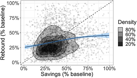
Figure 2. Density plot of 2014–2019 savings and rebound event sizes. Note: Blue line plots relationship fit by LOESS-smoothing (shading shows standard error of fit); savings and rebound, expressed as a percentage of baseline 2002–2012 water use; dotted line plots one-to-one linear relationship.
Download figure:
Standard image High-resolution image4.2. Survival analysis
Figure 3(A) plots a Kaplan–Meier curve for survival against effective rebound, stratified by residence type. Kaplan–Meier curves show the fraction of a population with no outcome at each time-step in their follow-up. The figure shows that—5 years after first conserving—only 25% of customers had effectively rebounded (i.e. increased consumption to an extent that reversed 75% or more of prior savings). Survival probabilities were significantly higher among customers in single-unit residences with outdoor space than in multi-unit residences with outdoor space, with lowest survival in multi-unit residences without outdoor space.

Figure 3. (A) Kaplan–Meier plot of conservation survival relative to the effective rebound outcome, stratified by residence type (Note: Crosses indicate time periods with censored observations). (B) Estimates and 95% confidence intervals (CIs) for mean survival against any and effective rebound, by customer type. (C) Estimates and 95% CIs of effects of customer characteristics on 2014–2015 conservation survival time, stratified by outcome (any rebound, effective rebound) and residence type. Note: Coefficients expressed in terms of their effect on the logarithm of survival time (t); coefficients not significant at the 5% level are whited-out; estimates and CIs are not shown for variables-outcome combinations with insufficient data.
Download figure:
Standard image High-resolution imageAs figure 3(B) shows, the curves fit by accelerated failure times models imply long survival times: for the whole sample, time to any rebound averaged 4.6–4.8 years; time to effective rebound averaged 7.6–8.3 years. For the average customer, this survival implies it has taken 5 years for water use to increase detectably after 2014–2015—and will take roughly 8 years for water use to effectively rebound to prior levels.
Figure 4 displays coefficients and 95% confidence intervals for the effect of customer-level variables on 2014–2015 conservation survival time, as measured by any or effective rebound. Since the water use behaviors of the four residence types are inherently different, we model the effects of customer-level variables on them separately. For single- and multi-unit customers with outdoor space, the results show large conservation events (as a fraction of baseline water consumption) generally have a substantially longer time to effective rebound, reinforcing our previous finding that rebounding customers who conserved more were less likely to reverse prior savings. This effect is generally inverted, however, for any rebound: a 10% increase in relative conservation is associated with a 2%–3% decrease in time to any rebound—probably reflecting a greater likelihood that water consumption will adjust upwards after a drastic reductions.

Figure 4. (A) Estimates and 95% confidence intervals of effects of block-group level demographic characteristics on 2014–2015 conservation survival time, stratified by outcome (Note: Coefficients expressed in terms of their effect on the logarithm of survival time t, coefficients not significant at the 5% level are whited-out). (B) Precinct-level vote shares received by Hilary Clinton in the 2016 election overlayed with conservation survival time 'hot' and 'cold' spots in Mesa Water's service area (Note: Hot and cold spots measured by Getis-Ord GI* statistic; contour lines for hot-spot densities computed by 2D kernel density smoothing).
Download figure:
Standard image High-resolution imageFor single family customers with indoor and outdoor space, two other customer characteristics also significantly associate with conservation survival. First, higher baseline water consumption associates with greater survival against effective rebound, meaning conserving customers with higher baseline consumption were more likely to continue conserving water (which may reflect the impact of customer affluence, roughly proxied of average water use). Second, occupancy changes negatively associate with time to effective rebound, suggesting occupancy changes lead to other changes (e.g. landscaping, remodeling) that increase consumption.
Figure 4 shows water use efficiency rebates during follow-up are not significantly associated with survival against either type of rebound. This may be due to the small number of efficiency rebates in 2015–2019: only 30 among 6062 single indoor and outdoor customers with detected conservation in 2015–2016. Indeed, there were not enough observations to estimate the impact of efficiency rebates on indoor-only single- and multi-unit customers (hence their omission from figure 4).
Figure 5(A) shows how neighborhood-level demographic covariates correlate with conservation survival time—after accounting for the above customer-level effects. We included four demographic covariates measured at the level of U.S. census block-groups: median household income, median age, share of owner-occupied residences, and share of married households. In addition, we included the precinct-level share of votes received by Hillary Clinton, the 2016 U.S. Democratic presidential candidate.
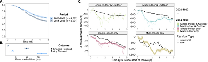
Figure 5. (A) Kaplan–Meier plot of conservation survival relative to the effective rebound outcome, stratified by detection period: 2008–2009 and 2014–2015 (Note: Crosses indicate time periods with censored observations). (B) Estimates and 95% confidence intervals (CIs) for mean survival against any and effective rebound, by detection period: 2008–2009 and 2014–2015. (C) Mean residual water use changes relative to each follow-up period's start, stratified by residence type; solid colored lines and ribbons show means and 95% CIs for 2014–2018 'structural' changes in consumption residuals identified by consumption change detection, dashed colored lines show mean 'raw' consumption residual; for reference, black lines plot each customer type's mean 2008–2012 structural water use change from January–February 2008.
Download figure:
Standard image High-resolution image
Results show median household income and the share of married households do not correlate significantly with time to either type of rebound. However, higher owner-occupied residence share and lower median age are both associated with greater survival against both types of rebound. As showcased in figure 5(B), the precinct-level share of Democratic votes associates positively with survival time against effective rebound, suggesting cultural and political factors were important in determining behaviors relevant to environmental actions and therefore conservation persistence.
4.3. A tale of two droughts
We compare conservation survival in California's most recent (2012–2016) drought to the less severe 2007–2009 drought. Specifically, we compare conservation events detected in 2014 and 2015 to ones detected in 2008 or 2009, following conserving customers for 3–5 years.
Conservation was somewhat more persistent in 2008–2009 than it was in 2014–2015 (figure 5(A)). Average implied survival against effective rebound is 9.8–11.5 years for 2008–2009 conservation, 2–3.5 years longer than the survival time observed 2014–2015 conservation (panel (B)); survival against any rebound tells a similar story: survival times are 0.5–1 years longer in 2008–2009 than in 2014–2015. This suggests heightened public awareness and media coverage in 2014–2015 lead to increased but less persistent conservation than in the 2007–2009 drought. Note that this comparison does not isolate the effects of public awareness associated with severe droughts—the 2007–2009 economic recession may have limited water consumption growth (and rebound) after 2009, for example. At the very least, it provides no evidence that 2014–2015 conservation persisted longer than in 2008–2009.
Figure 5(C) explores one potential reason for the difference in conservation persistence. The figure shows changes in average raw and structural components of each customer type's water use residual. The raw component is the deviation of consumption from its predicted value obtained in the first step of consumption change detection. The structural component is the step function fit to the raw residual in the second step of consumption change detection, capturing all conservation and rebound events detected during the 5 year drought period.
Figure 5(C) shows that 2012–2016 drought's climax produced steep consumption reductions among customers with outdoor water use. Short-term consumption responses captured by raw residual changes (plotted as dotted, colored lines) shows precipitous declines into mid-2015, when California introduced the first statewide mandatory outdoor watering restrictions. A sizable share of these reductions disappears by year's end, however. More moderate declines in structural residuals persist for longer but are partially reversed over the next two years, such that structural savings 5 years after the drought's beginning are similar in 2012–2016 as in 2008–2012. Thus, although the 2012–2016 drought produced relatively deep consumption reductions among customers with outdoor watering, these were likely associated with more temporary behaviors (e.g. compliance with outdoor watering restrictions) that ended as dry conditions eased.
The evolution of consumption residuals is somewhat different among customers without outdoor watering. In single-unit residences, there is a less pronounced trough in raw and structural consumption residuals in mid-2015, after which residuals rise slightly before declining once more post-2017. The structural consumption residual change of customers in multi-unit residences reaches its minimum in mid-2016, with only a slight increase by the end of 2019. In both cases, water savings after 5 years are indistinguishable from those achieved after January 2008.
5. Discussion
This study introduces a novel approach combining the methodological strengths of change detection and survival models to analyze customer-level conservation persistence after California's severe 2012–2016 drought. We find that—of the 52% of residences with detected water conservation in 2014 or 2015—roughly 25% had effectively rebounded to prior consumption levels after 5 years (i.e. had increased consumption to an extent that reversed at least 75% of prior water savings), implying average conservation survival of roughly 8 years. Larger conservation events survived longer, whereas conservation events in residences with an occupancy change during follow-up—survived for less time. A neighborhood's age and political inclination were also important: younger and more progressive areas had more persistent conservation. Despite the long conservation survival times identified, we do not find that the more severe 2012–2016 drought led to more persistent savings than the 2008–2010 drought; instead, its salience and heightened public awareness likely produced an extra surge in temporary conservation behavior that evaporated as the drought receded.
This study contributes a systematic method for customer-level analysis of conservation and rebound associated with a drought, a unique climatic episode where policy and media stressors exert an important external influence on water use [24, 25]. We note that—since these are externally determined—control-group comparisons are generally unavailable to infer their impact on water use behavior and our results should be interpreted accordingly. The change detection method employed here uses ensemble learning on prior data, controlling for water tariffs, weather, and economic effects to construct counterfactual water use for each customer [24]. But this method does not disentangle the effects of external drivers (e.g. California's May 2015 mandatory urban watering restriction) from Mesa Water's drought policy initiatives. Analyses of multiple utilities with different responses to drought conditions could elucidate which local policy interventions help drive conservation persistence during a drought—instead of just the regional policies and weather factors that drive drought 'awareness'. Similarly, our comparison of the 2007–2009 and 2012–2016 droughts is merely descriptive, at most presenting an absence of evidence that the 2012–2016 drought led to more persistent water savings than the 2007–2009 drought—not evidence of absence of the same finding.
Despite these caveats, our analysis is broadly consistent with prior work on conservation persistence in an experimental setting where conservation can be inferred using control group comparisons: customer feedback interventions. Alcott & Rogers, for example, analyze the long-term response of electricity customers to home energy reports and find that their effect decays 10%–20% yr−1 after the end of treatment, implying a similar conservation survival time as this study [31]. For water use, user feedback's effect seems to be shorter-lived, with studies finding treatment effects decay to 1/3 of their original size [14] or are undetectable one year after treatment [48]. But estimated treatment effects of water customer feedback in these studies are small, averaging just 5%–10% of baseline water use [14, 48], as opposed to the 30%–40% savings we detected in 2014–2015. Our contribution to existing work on conservation persistence is thus that the drought context—and its associated local and regional savings campaigns, media coverage, policy initiatives, and heightened public awareness—is likely to induce deeper and more prolonged water savings than customer feedback alone.
This finding has broader implications for water supply and demand management in a globalized world where climate-related water supply shocks are likely to become more frequent—even as demand is buffeted by multiple external socio-economic and environmental stressors. In this environment, scalable customer analytics tools enable utilities to discern and disentangle demand management's potential value streams. We have seen a severe drought can induce widespread and drastic water use reductions, which helps insure against short-term supply shortages. If such year-to-year 'demand response' is accompanied by decisions to improve the water efficiency of residential appliances or landscaping, it can also provide a longer-term infrastructure efficiency service that extends available water supplies.
Determining the behavior-infrastructure balance of observed water use changes is critical to understanding which service customers are providing. The difference is, in turn, important for long-term planning. A neighborhood with more permanent water savings may be less capable of drastic water use reductions in the future (e.g. because landscaping changes limit the impact of outdoor watering restrictions). Although not included here for brevity, analysis of conservation behavior across the two drought periods does not show that customers with prior conservation in 2008–2012 had differing levels of conservation persistence in 2014–2014. Nonetheless, the likelihood of conservation 2014–2018 was significantly lower among this subgroup—supporting the 'demand hardening' hypothesis in which water savings limit the capacity for future conservation as customers exhaust low-cost savings alternatives [49] (details of both analyses are given in the SI). This last finding underscores the need to account for the persistent impacts of prior drought episodes on future conservation behavior, which may be mediated by long-term processes like social memory or changes to residential infrastructure [39].
Regardless of the capacity for future water savings, prior savings persistence should be incorporated into demand forecasts and infrastructure planning decisions. For example, water supply planners can use more nuanced water demand models by treating conservation as a survival process in drought scenario analyses—using parameters tuned to a specific service area. Survival analyses of past droughts might also reveal what long-term demand responses are likely in the future. Our results show that both drought periods (2007–2009 and 2012–2016) were associated with net demand reductions that stabilized at 10% after 5 years and savings that persisted for more than 8 years. This knowledge could help Mesa Water determine the adequacy of its current water supply portfolio 10–15 into the future.
Top-down evaluation tools like the one proposed here also allow utilities to infer permanent water use reductions—a valuable use-case when customer turf replacement or appliance upgrade are not tracked by utility-administered rebate programs. Although published estimates of such untracked efficiency upgrades are not generally available, they may be quite common. In one analysis, for example, Mesa Water found that rebates accounted for just one-third of smart irrigation controllers registered by the manufacturer in its service area [50]. Indeed, rebates' limited ability to identify all efficiency upgrades is consistent with our finding that they were not associated with more persistent conservation outcomes. More research is thus needed to better understand what drives customer decisions to improve their household's water use efficiency and what the ultimate impact of those decisions is.
What is clear from this study is that the collective decisions of customers can have long-term water demand implications—whether they consist of upgrades to the distributed technologies that dispense water for end use, or persistent shifts in consumption habits. In either case, customers are integral to the infrastructure systems that serve them. As research has shown, their actions are sensitive to a multitude of internal and external factors that can influence behavior in a globalized, interconnected world [24, 25]. Tracking their short- and long-term responses to these factors is necessary for any sound infrastructure management strategy.
Acknowledgments
We gratefully acknowledge the Woods Institute for the Environment, Environmental Venture Projects program for funding this research. We would also like to thank Stefan Wager at the Stanford Graduate School of Business, Kim Quesnel at the Bill Lane Center for the American West, Philip Womble at the Woods Institute for the Environment, and Kristin Sainani at Stanford's Epidemiology and Public Health Department—for valuable feedback on this work.
Data availability statement
The data that support the findings of this study are available upon request from the authors. Raw customer billing data are not publicly available because the authors have signed a non-disclosure agreement with the utility partner for this study (Mesa Water District).
The data generated and/or analysed during the current study are not publicly available for legal/ethical reasons but are available from the corresponding author on reasonable request.
Author contributions
J B was responsible for data analysis, study conceptualization and writing the manuscript. N A contributed the customer billing data and rigorously reviewed/edited the manuscript draft. R R reviewed the manuscript and provided feedback. N A and R R also worked closely with J B to conceptualize the study.
Conflict of interest
The authors declare no competing interests.
Supplementary data (1.2 MB DOCX)