

Abstract
Global estimates of the land carbon sink are often based on simulations by terrestrial biosphere models (TBMs). The use of a large number of models that differ in their underlying hypotheses, structure and parameters is one way to assess the uncertainty in the historical land carbon sink. Here we show that the atmospheric forcing datasets used to drive these TBMs represent a significant source of uncertainty that is currently not systematically accounted for in land carbon cycle evaluations. We present results from three TBMs each forced with three different historical atmospheric forcing reconstructions over the period 1850–2015. We perform an analysis of variance to quantify the relative uncertainty in carbon fluxes arising from the models themselves, atmospheric forcing, and model-forcing interactions. We find that atmospheric forcing in this set of simulations plays a dominant role on uncertainties in global gross primary productivity (GPP) (75% of variability) and autotrophic respiration (90%), and a significant but reduced role on net primary productivity and heterotrophic respiration (30%). Atmospheric forcing is the dominant driver (52%) of variability for the net ecosystem exchange flux, defined as the difference between GPP and respiration (both autotrophic and heterotrophic respiration). In contrast, for wildfire-driven carbon emissions model uncertainties dominate and, as a result, model uncertainties dominate for net ecosystem productivity. At regional scales, the contribution of atmospheric forcing to uncertainty shows a very heterogeneous pattern and is smaller on average than at the global scale. We find that this difference in the relative importance of forcing uncertainty between global and regional scales is related to large differences in regional model flux estimates, which partially offset each other when integrated globally, while the flux differences driven by forcing are mainly consistent across the world and therefore add up to a larger fractional contribution to global uncertainty.
Export citation and abstract BibTeX RIS

Original content from this work may be used under the terms of the Creative Commons Attribution 4.0 license. Any further distribution of this work must maintain attribution to the author(s) and the title of the work, journal citation and DOI.
1. Introduction
During the last decade, about 45% of anthropogenic carbon dioxide (CO2) emissions remained and accumulated in the atmosphere. Model- and observation-based studies suggest that the remaining term was shared among ocean (24%) and land (32%) since 1960 (Friedlingstein et al
2021). Together, the contribution of the ocean and terrestrial CO2 uptake nearly halves the increase in atmospheric CO2, damping the pace of climate change (Canadell et al
2021). These sinks significantly increased since the middle of the 20th century, mainly due to the acceleration of the increase in CO2 concentrations, caused by fossil fuel emissions. However, carbon uptake processes depend strongly on climate variability, especially for the terrestrial biosphere (Le Quéré et al
2009, DeVries et al
2019). While the ocean sink grew from  PgC·yr−1 in the 1960s to
  PgC·yr−1 in 2011–2020, with an inter-annual variability of a few tenths of PgC·yr−1, the land sink rose from
  PgC·yr−1 to
  PgC·yr−1, but with inter-annual variations up to 2 PgC·yr−1 (Friedlingstein et al
2021).
PgC·yr−1, but with inter-annual variations up to 2 PgC·yr−1 (Friedlingstein et al
2021).
Accurate evaluations of anthropogenic emissions, atmospheric CO2 levels and carbon cycle perturbation are necessary to monitor, understand and predict climate change. The Global Carbon Project (GCP) has published an annual report since 2013 (Le Quéré et al
2013, 2014, Friedlingstein et al
2020, 2021) that quantifies the magnitude and uncertainty of the five major components of the global carbon budget: fossil fuel emissions ( ), emissions from land use change (
 ), the growth rate of atmospheric CO2 (
 ), the ocean sink (
 ) and the land sink (
 ). In earlier analyses provided by the GCP, the terrestrial carbon cycle simulated by the terrestrial biosphere models (TBMs, called by the authors Land Biosphere Models or Dynamical Global Vegetation Models) was not considered reliable enough to be used in the report to estimate the land carbon sink (Le Quéré et al
2009, Schaefer et al
2012, Todd-Brown et al
2013). The land sink
). In earlier analyses provided by the GCP, the terrestrial carbon cycle simulated by the terrestrial biosphere models (TBMs, called by the authors Land Biosphere Models or Dynamical Global Vegetation Models) was not considered reliable enough to be used in the report to estimate the land carbon sink (Le Quéré et al
2009, Schaefer et al
2012, Todd-Brown et al
2013). The land sink  was hence diagnosed indirectly as the residual of the other terms. However, the methodology was updated in the 2017 global carbon budget (Le Quéré et al
2017), partly due to improvements in carbon cycle representation (Collier et al
2018, Lawrence et al
2019, Arora et al
2020, Davies-Barnard et al
2020), but also because of evidence of underestimation and uncertainty in the ocean sink variability (Landschützer et al
2015, DeVries et al
2017). The global land sink is now estimated by the multi-model mean of the TBM simulations, with the budget imbalance term,
was hence diagnosed indirectly as the residual of the other terms. However, the methodology was updated in the 2017 global carbon budget (Le Quéré et al
2017), partly due to improvements in carbon cycle representation (Collier et al
2018, Lawrence et al
2019, Arora et al
2020, Davies-Barnard et al
2020), but also because of evidence of underestimation and uncertainty in the ocean sink variability (Landschützer et al
2015, DeVries et al
2017). The global land sink is now estimated by the multi-model mean of the TBM simulations, with the budget imbalance term,  , representing residual uncertainty and/or unexplained aspects of the actual global carbon cycle.
To account for model construction, structural, and parametric uncertainty, as many as 17 TBMs were used to estimate  by (Friedlingstein et al
2020). Simulations were run using a unified land use change data set (LUH2; Hurtt et al
2020), global atmospheric CO2 trend, and atmospheric climate forcing (CRUJRA; Harris 2019). Use of a single forcing dataset for climatic forcing, however, means that any model spread due to climate forcing data uncertainty is not represented by the GCP ensemble. Yet, several studies have identified historical climate forcing as a large source of uncertainty in terrestrial carbon cycle modelling (Hicke 2005, Jung et al
2007, Poulter et al
2011, Bonan et al
2019, Lawrence et al
2019). Hicke (2005), for example, highlights important biases in net primary productivity (NPP) estimation while using different radiation datasets, and (Poulter et al
2011) conclude that atmospheric forcing results in a large uncertainty compared to land-cover datasets for NPP, heterotrophic respiration (Rh) and net ecosystem exchange. More recently, as part of the assessment and benchmarking of the Community Land Model version 5 (CLM5) (Lawrence et al
2019), climate forcing uncertainty was compared to model structure uncertainty using two forcing data sets (Global Soil Wetness Project 3 and CRUNCEP) and three versions of CLM (CLM4, CLM4.5, and CLM5) that differ markedly in their carbon cycle representation (Bonan et al
2019). The authors concluded that climate forcing is a large source of uncertainty in the global carbon cycle, especially for GPP, NPP and Rh, and to a lesser extent for Net Biome Productivity. However, this study was performed with different versions of a single model, and only two estimates of atmospheric climate forcing. Arguably therefore, the importance of atmospheric forcing on carbon cycle estimation by TBMs remain insufficiently explored, especially in the context of recent model structural improvements in the 6th Coupled Model Intercomparison Project (CMIP6) generation of models.
by (Friedlingstein et al
2020). Simulations were run using a unified land use change data set (LUH2; Hurtt et al
2020), global atmospheric CO2 trend, and atmospheric climate forcing (CRUJRA; Harris 2019). Use of a single forcing dataset for climatic forcing, however, means that any model spread due to climate forcing data uncertainty is not represented by the GCP ensemble. Yet, several studies have identified historical climate forcing as a large source of uncertainty in terrestrial carbon cycle modelling (Hicke 2005, Jung et al
2007, Poulter et al
2011, Bonan et al
2019, Lawrence et al
2019). Hicke (2005), for example, highlights important biases in net primary productivity (NPP) estimation while using different radiation datasets, and (Poulter et al
2011) conclude that atmospheric forcing results in a large uncertainty compared to land-cover datasets for NPP, heterotrophic respiration (Rh) and net ecosystem exchange. More recently, as part of the assessment and benchmarking of the Community Land Model version 5 (CLM5) (Lawrence et al
2019), climate forcing uncertainty was compared to model structure uncertainty using two forcing data sets (Global Soil Wetness Project 3 and CRUNCEP) and three versions of CLM (CLM4, CLM4.5, and CLM5) that differ markedly in their carbon cycle representation (Bonan et al
2019). The authors concluded that climate forcing is a large source of uncertainty in the global carbon cycle, especially for GPP, NPP and Rh, and to a lesser extent for Net Biome Productivity. However, this study was performed with different versions of a single model, and only two estimates of atmospheric climate forcing. Arguably therefore, the importance of atmospheric forcing on carbon cycle estimation by TBMs remain insufficiently explored, especially in the context of recent model structural improvements in the 6th Coupled Model Intercomparison Project (CMIP6) generation of models.
In this study, we used the output from the TBMs of three Earth System Models (ESMs) participating in the CMIP6. We performed an analysis of variance similar to Hawkins and Sutton (2009), Lovenduski and Bonan (2017), Bonan et al (2019)in order to quantify the relative uncertainty from atmospheric forcing, models and forcing-model interactions in carbon flux estimates made by TBMs. We used a combination of three TBMs from ESM and three atmospheric forcing datasets in our analysis. We present results for the major terrestrial carbon cycle fluxes; gross primary productivity (GPP), autotrophic respiration (Ra) and heterotrophic respiration (Rh), at global and regional scales. We also investigate estimates of CO2 emissions from natural fires (fFire) and highlight their role in the calculation of the land carbon sink, before focusing on sources of uncertainty in the global net ecosystem productivity (NEP = GPP−Ra−Rh−fFire).
2. Methods
2.1. CMIP6 models and atmospheric forcings
We used the results of three TBMs of CMIP6 ESMs described in table 1, from the Land Surface, Snow and Soil moisture Model Intercomparison Project (LS3MIP, Van den Hurk et al 2016) of CMIP6. For the three models, land use transitions are forced by the Land Use Harmonization 2 (LUH2) time series (Hurtt et al 2020). Those three models have been selected because they are the only ones that report output from three different atmospheric forcings and also share data for emissions from fire, on the Earth System Grid Federation archive.
Table 1. Model description.
| Terrestrial biosphere model | Community Land model CLM5 (Lawrence et al 2019) | ISBA-CTRIP (Decharme et al 2019, Delire et al 2020) | JSBACH3.2 (Reick et al 2021) |
|---|---|---|---|
| Parent climate model | Community Earth system model CESM2 (Danabasoglu et al 2020) | CNRM-ESM2-1 (Séférian et al 2019) | MPI-ESM1.2-LR (Mauritsen et al 2019) |
| Simulation resolution | 0.9∘ latitude by 1.25∘ longitude | T127 (∼1.4∘) | T63 (∼1.9∘) |
| Fire | Process-based (Li et al 2012, Li and Lawrence 2017) | Simple, based on GlobFirm (Thonicke et al 2001) | Mechanistic, SPITFIRE (Lasslop et al 2014) |
| Natural vegetation dynamics | No | No | Yes (Reick et al 2013) |
| Nitrogen cycle | Revised (Fisher et al 2019) | No | New (Goll et al 2017) |
| Plant hydrodynamics | (Kennedy et al 2019) | No | No |
| Soil carbon decompostion | Yes | Yes | New (Goll et al 2015) |
| Soil hydrology | Multilayer | Multilayer | Multilayer (Hagemann and Stacke 2015) |
| Other | Numerous updates to hydrology, snow, gas exchange and crops | Similar | Similar |
Three climate forcing datasets were used to force the TBMs, according to the LS3MIP protocol. Atmospheric forcing consists of hourly to 6 hourly data on precipitation, short and long wave solar radiation, near surface air temperature, specific humidity, and wind speed. The three forcings described in table 2 have a  spatial resolution.
Table 2. Atmospheric forcing description.
| Name | Global soil wetness project (GSWP3) version 1.09 (Kim 2017) | CRUJRA | Princeton (Sheffield et al 2006) v2.2 |
|---|---|---|---|
| Time resolution | 3 hourly | 6 hourly | 3 hourly |
| Covered period | 1901–2014 | 1901–2018 | 1901–2012 |
| Reanalysis used | 20th Century Reanalysis version 2 (Compo et al 2011) | Japanese Reanalysis (JRA) by the Japanese Meteorological Agency (JMA) | National Centers for Environmental Prediction (NCEP) reanalysis |
| Corrected by | |||
| air temperature | Climate Research Unit Timeseries (CRU TS) v3.21 | CRU TS v4.03 | CRU TS v3.2 |
| Precipitation | Global Precipitation Climatology Center (GPCC) v7 | CRU TS v4.03 | CRU, Global Precipitation Climatology Project and TRMM Multi-satellite Precipitation Analysis |
| Radiation | Surface Radiation Budget (SRB) datasets (downwelling radiation fluxes) | CRU TS v4.03 | SRB |
| Use | LS3MIP | GCP | Hydrology |
a Erroneously named CRUNCEP in CMIP6 simulations. b http://hydro.iis.u-tokyo.ac.jp/GSWP3/.
For reference, results of analysis of this set of model simulations with the International Land Model Benchmarking (ILAMB, Collier et al 2018) package are provided here: www.ilamb.org/land-hist/. ILAMB produces systematic evaluation (plots, summary tables, scoring) of model output against observations for a range of metrics including bias, RMSE, pattern correlation, annual cycle phase, and variable-to-variable comparisons. The version of ILAMB presented here assesses 22 land carbon, water, and energy cycle variables model variables against more than 50 observational datasets.
2.2. Analysis of variance
To statistically disaggregate the impacts of climate forcing, model choice and their interactions on relevant output variables, we performed an ANOVA. We analysed nine terrestrial carbon cycle simulations—three TBMs forced by three forcings—for the time period 1960–2012, chosen to coincide with the beginning of atmospheric carbon dioxide measurements in the 1960s, and the end of the Princeton dataset. We quantify relative uncertainty into three sources: models, atmospheric forcing differences and model-forcing interactions which measure the fact that models behave differently to different forcing product. Details can be found in the supplementary material.
3. Results
3.1. Global scale
We first investigated and compared the forcing data in order to highlight the main differences and similarities. The three forcings mostly agree on near surface air temperature, but they present large differences in specific humidity, incoming shortwave and longwave radiation, and windspeed (figure 1). Princeton has much higher specific (and relative—not shown) humidity than CRUJRA or GSWP3 in most parts of the world, except in desert areas. Additionally, specific humidity is generally greater with GSWP3 than with CRUJRA in tropical regions. CRUJRA also has higher shortwave and lower longwave incoming radiation than GSWP3 and Princeton, both having almost identical values. The precipitation forcing differs also with higher values for GSWP3, especially within the Arctic circle related to snowfall uncertainties.

Figure 1. Annual mean of atmospheric variables used to drive terrestrial biosphere models: GSWP3 (gswp, left-most column), Princeton minus GSWP3 (pgf-gswp; center left column), CRUJRA minus GSWP3 (crujra-gswp; center right column), and zonal averages of each product (right-most column).
Download figure:
Standard image High-resolution imageWe performed the analysis of variance on the global estimates of GPP, Ra, Rh, GPP–Ra–Rh, fFire and NEP (figure 2). The results illustrate a dominant role of the atmospheric forcing variation on global GPP estimates (figure 2(a)), with large differences between the multi-model mean values according to the forcings (about 15 PgC·yr−1), with GSWP3 resulting in lowest GPPs for all three models, Princeton the highest GPPs, and CRUJRA in between. The discrepancies between the models for a given forcing are smaller, especially for CRUJRA and Princeton. Global GPP estimates of the ISBA-CTRIP and CLM5 models are very similar when forced with the CRUJRA forcing, and slightly differ when forced with GSWP3 or Princeton. The global GPP estimates of JSBACH are the largest with all three forcings and the difference with the two other models is the biggest with the GSWP3 forcing. However, the three models obtain very similar results with the Princeton atmospheric forcing. This suggests a general sensitivity of the models to an atmospheric variable that is different between Princeton's and the two other forcings, such as specific humidity (figure 1). These nine simulation results indicate a strong sensitivity of modelled GPP to climate forcing.
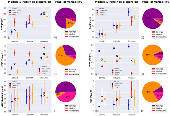
Figure 2. Model means and standard deviations (color dots and bars) and multi-model means (black crosses) of global carbon flux time series for each atmospheric forcing between 1960 and 2012 (pointplot) and fractional distribution of uncertainty (variability) obtained from the ratios of the sum of squared deviation from the mean (equations (3)–(6) in supplementary material) (pieplot) for GPP (a), (b), Ra (c), (d), NPP (e), (f), fFire (g), (h), GPP−Ra−Rh (i), (j) and NEP = GPP−Ra−Rh−fFire (k), (l). Standard deviations are calculated from the yearly time series of the fluxes.
Download figure:
Standard image High-resolution imageFigure 2(b) confirms the dominant role of atmospheric forcing on global GPP uncertainty. It accounts for ∼75% of the variability in the mean estimates, against ∼19% for models and ∼6% for interactions terms.
The dominance of atmospheric forcing contribution over the uncertainty is even more obvious for autotrophic respiration (figure 2(c)), again with similar model mean values for a given forcing but large differences between forcings with no overlap. According to our analysis of variance, ∼90% of the uncertainty can be assigned to forcings, ∼5% to models and ∼5% to the interactions terms (figure 2(d)). The Princeton forcing results in a slightly larger spread between the average autotrophic respiration than the other forcings.
Global NPP (GPP–Ra) behaves differently. Despite differences in multi-model mean values per atmospheric forcings (around 5 PgC·yr−1) attesting to the role of forcing in uncertainty, we can see that JSBACH estimates are clearly higher than the two others (more than 10 PgC·yr−1) in figure 2(e). This indicates greater model contribution to uncertainty, confirmed by figure 2(f) where models are the dominant source (∼63%) of uncertainty for NPP, but atmospheric forcing remains important with ∼30% of variability explained and ∼7% for model-forcing interactions. Contrary to ISBA-CTRIP and CLM5 that simulate the lowest NPP with GSWP3 and the highest with Princeton (like for GPP and Ra), JSBACH simulates a slightly smaller global NPP with the CRUJRA forcing. Global Rh presents similar results to global NPP (not shown), both for atmospheric contribution to uncertainty and for greater values obtained with GSWP3 than CRUJRA for JSBACH.
We show that atmospheric forcings have an important (NPP, Rh) and even dominant (GPP, Ra) role in uncertainty distribution for the major fluxes of global carbon cycle estimates. It seems that forcing contribution to uncertainty decreases when we consider net flux such as NPP and Rh rather than direct products of photosynthesis (GPP and Ra).
Wildfires are a small contribution to the global land carbon loss fluxes (∼2–3 PgC·yr−1) (Van der Werf et al 2010), especially when compared to plant and soil respiration. Nonetheless, fire carbon losses correspond to approximately one-third of the GPP–Ra–Rh net flux. Moreover, this flux has particularly high seasonal and inter-annual variability, in response to both land cover change, as well as climatic events like drought. Despite its importance, anthropogenic biomass burning is not yet represented by all TBMs. Overall, high uncertainty remains in the carbon emissions associated with fire (figures 2(g) and (h)). ISBA-CTRIP tends to overestimate global fire emissions compared to the global fire emission database (2.14 PgC·yr−1 for 1997–2015 van der Werf et al, 2017), while JSBACH is slightly lower (especially with Princeton). Part of these differences may be explained by the intermediate complexity fire module GlobFirm (Thonicke et al 2001) used in ISBA-CTRIP that is known to overestimate fire emissions (Li et al 2012). Figure 2(g) shows a large discrepancy between model values for a given forcing, particularly for the Princeton one, and figure 2(h) confirms a fractional contribution to uncertainty of ∼85% for the models, ∼6% for forcings and ∼9% for interactions. A closer look at fire results shows indeed interesting interactions between the forcings and fire modules that explain the bigger dispersion for Princeton. We saw that GPP and NPP (GPP–Ra) is enhanced with the Princeton forcing, most probably because of the high level of air humidity. For the GlobFirm module implemented in ISBA-CTRIP, this leads simply to lower evapotranspiration rates, less moisture stress, higher productivity and litterfall (not shown) resulting in more biomass burned and greater associated carbon emissions. However, with the more mechanistic fire module of CLM5, the higher air humidity results directly in lower level of fuel flammability (see equation (8) Li et al 2012). In JSBACH, finally, the three applied forcings cause very different fire-vegetation feedbacks, such that the natural vegetation cover in the three simulations differs strongly, particularly in fire prone regions such as Africa and Asia (not shown). Such strong fire-vegetation feedbacks have already been observed for JSBACH in previous idealised model simulations (Lasslop et al 2016). Emissions from fire appear to be quite sensitive to atmospheric forcing when we compare individually the relative dispersion for each model, but this dependency is overshadowed in this analysis by the even larger uncertainty related to the model structure.
Here, we first present results for GPP–Ra–Rh estimates. This flux takes into account the most important and probably best represented processes of the terrestrial biosphere carbon sink, by excluding fire emissions. As expected, this net flux is smaller and has larger interannual variability (standard deviation) relative to the mean than the gross fluxes GPP, Ra and Rh. Figure 2(i) suggests a more important contribution to uncertainty by forcing than models: model mean values are close to each other for a given forcing and there is a small difference between forcings. The analysis of variance results shows effectively a dominant role of forcings (∼52%) over models (∼8%) but also a substantial contribution of the interaction terms (∼40%) (figure 2(j)). Indeed, the models do not show similar patterns with respect to the forcings. CLM5 results in greater values for CRUJRA (6.53 PgC·yr−1) than Princeton (6.14 PgC·yr−1), while ISBA-CTRIP simulates slightly bigger fluxes with Princeton (6.33 PgC·yr−1) than with CRUJRA (6.23 PgC·yr−1), as does JSBACH with a greater difference (6.06 for CRUJRA against 6.68 PgC·yr−1 with Princeton). In addition, we observe only slightly bigger results for CRUJRA than GSWP3 for JSBACH, consistent with the results obtained from Rh and NPP, while the difference is more pronounced for ISBA-CTRIP and CLM5. This highlights differences in model sensitivity to atmospheric forcings, such as air humidity or downward radiation flux, for the land sink calculation.
Larger differences are obtained when we take into account fFire in the NEP calculation (figures 2(k) and (l)). There is only a small difference between the multi-model mean values per forcing, and a larger spread between the values of the different models, especially with the Princeton forcing (figure 2(k)). Moreover, global NEP is almost independent of the forcing with CLM5 and ISBA-CTRIP, which is not the case with JSBACH. The variance analysis results show that models contribute ∼75% to uncertainty, forcings account for ∼9% and interactions for ∼16%. This contrasts with the significant forcing contribution we obtained when not accounting for fFire, and indicates clearly a high model uncertainty related to fire emission.
To complete the global picture we analyze the contribution of atmospheric forcing to uncertainty in carbon stocks (figure 3). Atmospheric forcing plays a role in global carbon stock uncertainties but not a dominant one like for gross carbon fluxes. There are large differences in live (cVeg) and dead biomass (cLitter), and soil organic carbon content (cSoil) between multi-model means per forcing but the differences between models are even larger. The analysis of variance for cVeg shows that ∼26% of the uncertainty can be assigned to forcings, ∼67% to models and ∼7% to the interactions terms (figure 3(b)). For cLitter and cSoil, these numbers are respectively ∼20% and ∼9% for forcing, ∼68% and ∼81% for models and ∼13% and ∼10% for interactions (figures 3(d) and (f)). CLM5 and ISBA-CTRIP both simulate the smallest live and dead stocks with GSWP3 while JSBACH simulates the smallest stocks with CRUJRA(figures 3(a), (c) and (e)). Princeton results in the largest stocks with every model. Live biomass from CLM5 and ISBA-CTRIP are fairly similar while JSBACH's is lower. The litter reservoir is the highest with ISBA-CTRIP and the lowest with CLM5 while the soil carbon is the largest with CLM5 especially for CRUJRA and Princeton. The higher soil carbon content with CLM5 can be explained by the vertically discretized soil carbon module with deeper soils (down to a maximum of 8.5 m). In the case of ISBA-CTRIP and JSBACH the soil carbon reservoir only represents the carbon in the first meter.
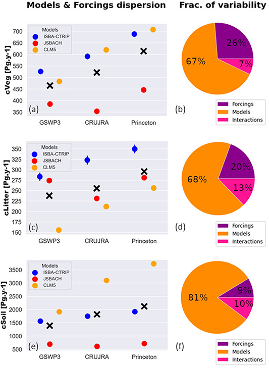
Figure 3. Model means and standard deviations (color dots and bars) and multi-model means (black crosses) of global carbon stocks time series for each atmospheric forcing between 1960 and 2012 (pointplot) and fractional distribution of uncertainty (variability) obtained from the ratios of the sum of squared deviation from the mean (equations (3)–(6) in supplementary material) (pieplot) for cVeg (a), (b), cLitter (including coarse woody debris) (c), (d), and cSoil (e), (f).
Download figure:
Standard image High-resolution image3.2. Regional scale
We performed the same analysis of variance on the 30 sub-continental regions defined in the Intergovernmental Panel on Climate Change (IPCC) Special Report on Managing the Risks of Extreme Events and Disasters to Advance Climate Change Adaptation (SREX; IPCC SREX 2012). Figure 4 presents the results for GPP, Ra and Rh. The regions that present the largest uncertainty (largest pies) for GPP (figure 4(a) and supplementary tables S2–S4) are North Asia (NAS), the Amazon forest (AMZ), and to a lesser extent West Africa (WAF), South Asia (SAS), South East Asia (SEA), East Africa (EAF), South Africa (SAF), and West North America (WNA) even if WNA contributes only 2–4 PgC·yr−1 to global GPP. Atmospheric forcing is a dominant source of uncertainty (more than half) in some regions that have fairly large contributions to the global total GPP flux, such as EAF and East Asia (EAS), but also in Central North America (CNA), West Coast South America (WSA), and North East Brazil (NEB). Atmospheric forcing is an important source of uncertainty (more than a third) in AMZ and WAF, tropical forest regions, which contribute greatly to global GPP. Generally, it seems that atmospheric forcings play an important role in tropical regions. Less important contribution in SAS and SEA could be explained by monsoon regimes that prevail on atmospheric forcing differences, but also by model resolution that could explain dominant model uncertainty in island regions (SEA but also Caribbean and Pacific Island Regions). Model-forcing interactions play a secondary but significant role in some regions such as NAS, WAF and South East South America (SSA) for the ones that contribute the most to global GPP.

Figure 4. Regional carbon fluxes for 1960–2012. Total flux value for each SREX region in background, distribution of uncertainty between forcings, models and interactions as overlayed pieplots with size of the pies proportional to the total uncertainty value (equation (3) and tables S2–S4 in supplementary material).
Download figure:
Standard image High-resolution image
Slightly different results can be observed for Ra (figure 4(b)). Atmospheric forcing contribution to uncertainty is lower in NAS and AMZ, as well as SEA and NEB. Generally, the forcing and interaction terms seem to play a less important role in Ra than in GPP regional estimates. For Rh (figure 4(c)), forcing contribution is even more reduced in tropical regions, where the fractional distribution never exceeds one-third. However, atmospheric forcing plays an important role in heterotrophic respiration uncertainty in the northern hemisphere's mid and high latitudes (about one-third). Interaction terms become also important in numerous mid and northern regions, particularly in NAS, CNA and Central Europe (CEU). An interpretation could be that models do not predict the same evolution for Rh in the areas where atmospheric variables are changing faster.
It is interesting to probe why atmospheric forcing accounts for more uncertainty at global than regional scale. We found that some differences between the forcings have the same impact on most of the world's area, while model differences induce strong regional uncertainty but not in the same manner everywhere. As an example, GPP estimates are slightly larger with Princeton than with CRUJRA or GSWP3 in all regions (see supplementary material figure S1), regardless of the model and add up to a large difference at global scale. This is consistent with the idea that the higher humidity in the Princeton dataset allows for higher photosynthetic rates for all models forced by it. Conversely, GPP estimates by ISBA-CTRIP and CLM5 appear to be similar at global scale, yet the regional analysis highlights strong opposition between tropical regions with higher GPP for ISBA-CTRIP compared to CLM5, and the northern hemisphere which has higher GPP in CLM5 compared to ISBA-CTRIP (see supplementary material figure S2). This leads to a strong model contribution to uncertainty at regional scale, but those differences compensate each other globally.
4. Conclusion
The goal of this study was to evaluate the uncertainty related to the use of different global atmospheric forcing datasets in terrestrial carbon cycle modelling. We used nine CMIP6 simulations from three TBMs run with three different forcings to perform our analysis. First, we focused on global averages and found that atmospheric forcings are a dominant source of uncertainty compared to model choice for GPP and Ra, and contribute significantly to the overall uncertainty for Rh and NPP. The contribution of atmospheric forcing to the net fluxes uncertainty is reduced since positive effects of atmospheric forcings on photosynthesis are partially offset by enhancement in the respiration fluxes. We still found an important role of atmospheric forcing on GPP-Ra-Rh temporal mean estimates, but with important interaction terms that translate different model responses to climate variables. Important differences in fire modelling lead to a dominant role of models in NEP uncertainty, even on a global scale, despite a visible relationship and interactions between fire emission and climate forcings.
Secondly, we looked at the partitioning of uncertainty at the regional scale, with the purpose of identifying the regions where atmospheric forcings contribute the most to the variability of GPP, Ra and Rh. We showed that generally, the model structure is the dominant source of uncertainty regionally, in contrast to what we found globally. Atmospheric forcing contribution remains significant and even slightly dominant in some regions, notably in tropical forests for GPP and Ra and in mid and northern high latitudes for Rh, but regional discrepancies among the models are stronger. However, and in contrast with the forcings, it is not the same models that result in the biggest and lowest values everywhere. Those differences add up and offset each other, leading to closer results globally.
While the purpose of the study was to investigate the contribution of forcing uncertainty and to demonstrate the influence of choosing a specific forcing over another forcing, this experimental design, using three distinct sets of forcing data fields is not ideal for identifying the relative sensitivity to which drivers are most critical. While the large difference in humidity between Princeton and the other two datasets points to that field being particularly important in governing GPP and other fluxes, a more specific one-at-a-time propagation of the uncertainty in each field may allow for a more specific attribution of uncertainty to meteorologic variables. Likewise, perturbations to the distributions while holding mean values constant may allow attribution of carbon cycle sensitivity to extremes. Nonetheless, these results point to a focus on constraining humidity values as key to reducing forcing uncertainty. To the extent that humidity is a key driver in GPP uncertainty, another question is whether this uncertainty is exacerbated in offline simulations such as used here, GCP, and elsewhere, because of the inability for surface moisture fluxes to attenuate humidity biases in the forcing fields due to the one-way coupling.
Additional work involving more TBMs and climate forcings should be done in order to better quantify the role of forcings in carbon cycle uncertainty, especially for the interactions between fire, land-cover dynamics and climate forcings. Even so, we conclude that atmospheric forcings are a key source of uncertainty in carbon cycle modelling at the global scale and are a significant source of uncertainty in some regions. Therefore, we suggest that where possible, it would be preferable for future MIPs and assessments (e.g. TRENDY, GCP, CMIP) to run simulations with several alternative climate forcing datasets, and to more specifically generate datasets to allow attribution of carbon cycle sensitivity both to uncertainty in meteorologic fields and to uncertainty in mean versus extreme values of meteorologic fields, when estimating the terrestrial carbon sink in order to correctly represent the uncertainty associated.
Data availability statement
The data that support the findings of this study are openly available at the following URL/DOI: https://esgf-node.llnl.gov/search/cmip6/.
Acknowledgments
L H, C D, B D, R S, T S and R F acknowledge funding by the European Union's Horizon 2020 (H2020) research and innovation program under Grant Agreement No. 641816 (CRESCENDO) for L H, B D, C D and T S, No. 101003536 (ESM2025 – Earth System Models for the Future) for R S and No. 821003 (4C) for R F. C D and B D are supported by the 'Centre National de Recherches Météorologiques' (CNRM) of Météo-France and the 'Centre National de la Recherche Scientifique' (CNRS) of the French research ministry. D M L is supported by the National Center for Atmospheric Research, which is a major facility sponsored by the NSF under Cooperative Agreement 1852977 and by the U.S. Department of Energy, Office of Biological and Environmental Research Grant DE-FC03-97ER62402/A0101. J E M S N and T S would like to thank Veronika Gayler for conducting many of the CMIP6 MPI-ESM1.2-LR simulations. T S work was funded by the EU CRESCENDO Project. C D K acknowledges support by the Director, Office of Science, Office of Biological and Environmental Research of the U.S. Department of Energy under Contract DE-AC02-05CH11231 through the Early Career Research Program and the Regional and Global Model Analysis Program (RUBISCO SFA).
Supplementary data (1.8 MB PDF)