

Abstract
Climate projections are uncertain; this uncertainty is costly and impedes progress on climate policy. This uncertainty is primarily parametric (what numbers do we plug into our equations?), structural (what equations do we use in the first place?), and due to internal variability (natural variability intrinsic to the climate system). The former and latter are straightforward to characterise in principle, though may be computationally intensive for complex climate models. The second is more challenging to characterise and is therefore often ignored. We developed a Bayesian approach to quantify structural uncertainty in climate projections, using the idealised energy-balance model representations of climate physics that underpin many economists' integrated assessment models (IAMs) (and therefore their policy recommendations). We define a model selection parameter, which switches on one of a suite of proposed climate nonlinearities and multidecadal climate feedbacks. We find that a model with a temperature-dependent climate feedback is most consistent with global mean surface temperature observations, but that the sign of the temperature-dependence is opposite of what Earth system models suggest. This difference of sign is likely due to the assumption tha the recent pattern effect can be represented as a temperature dependence. Moreover, models other than the most likely one contain a majority of the posterior probability, indicating that structural uncertainty is important for climate projections. Indeed, in projections using shared socioeconomic pathways similar to current emissions reductions targets, structural uncertainty dwarfs parametric uncertainty in temperature. Consequently, structural uncertainty dominates overall non-socioeconomic uncertainty in economic projections of climate change damages, as estimated from a simple temperature-to-damages calculation. These results indicate that considering structural uncertainty is crucial for IAMs in particular, and for climate projections in general.
Export citation and abstract BibTeX RIS

Original content from this work may be used under the terms of the Creative Commons Attribution 4.0 license. Any further distribution of this work must maintain attribution to the author(s) and the title of the work, journal citation and DOI.
1. Introduction
Anthropogenic emissions increase the concentration of greenhouse gases in the atmosphere, resulting in radiative forcing F (W m−2) on the Earth system. The response of Earth's global mean surface temperature T (∘C, defined as an anomaly from a preindustrial baseline) to this forcing has been highly uncertain [1, 2] and will likely continue to be so. This uncertainty hampers the design and implementation of appropriate climate planning and policies, which costs on the order of trillions of dollars [3]. A core objective of modern Earth system research is thus to improve climate change projections. Earth's climate system is extraordinarily complex and mulitfaceted, meaning there are myriad sources of uncertainty. On the one hand, very complex Earth system models (ESMs), which attempt to represent as many of these processes as possible, are too computationally expensive to gauge how uncertainties propagate into uncertainty in T or other properties of interest. Thus the Intergovernmental Panel on Climate Change largely relies upon a heuristic characterisation of uncertainties [2]. On the other hand, simpler models of climate physics, such as the energy balance models (EBMs) used within the integrated assessment models (IAMs) of economists [4], or efficient reduced-complexity ESMs [5], can produce large ensembles of simulations, intended to characterise the uncertainty of the climate's response to a particular forcing or emissions trajectory. While ESMs are typically the core tool for of climate science projections such as in [2], EBMs are used to emulate ESMs, to explore alternative scenarios, assess parametric uncertainty and the economic impacts of internal variability, constrain with observations, and to represent climate physics within climate economics; thus both model frameworks are fundamentally important in guiding climate policy.
Large ensembles of climate model simulations tend to quantify parametric uncertainty—uncertainty of the model response to emissions associated with the numerical values of parameters used in these models [5]—and uncertainty due to internal variability—the natural variability intrinsic the climate system [6]. Another type of uncertainty, which is rarely quantified because it is more difficult to do so, is structural uncertainty—uncertainty of the model response to emissions associated with not being certain what equations to use for these models in the first place. Models along the entire axis of complexity are subject to structural uncertainty for different reasons; ESMs have many equations, some of which are derived from first principles and thus known with certainty but many of which are not, while Earth's climate is represented by simpler sets of equations in EBMs and IAMs, which thus may be less adequate for representing complex Earth system processes. Therefore, structural uncertainty may increase or decrease with model complexity, and may either dwarf or be negligible compared to parametric uncertainty and/or internal variability; this is unknown because of the lack of quantitative characterisation of structural uncertainty in climate models across the full axis of complexity. Structural uncertainty is heuristically and qualitatively captured by model intercomparisons such as CMIP [7], but these are necessarily qualitative and coarse characterisations of structural uncertainty. While quantifying structural uncertainty for ESMs is no less challenging due to computational limitations, EBMs and IAMs for which structural uncertainty has been neglected do not suffer this limitation.
We note that in a climate modelling context uncertainty is sometimes grouped into forcing uncertainty, model response uncertainty, and internal variability [8, 9], but that from a general uncertainty quantification perspective as we adopt here, both forcing and model response uncertainty involve both parameteric and structural uncertainty components. In other words, uncertainties are involved in both the parameters and equations that one uses to represent both the forcing on, and response of, the climate system. Furthermore, we note that internal variability emerges naturally from the interactions of different components of complex climate models, but can also be included in simple EBMs via stochastic terms; as the impact of internal variability on climate and economic projections in EBMs has been quantified elsewhere [10], here we focus on structural uncertainty.
Here we present a means to quantify structural uncertainty in a simple EBM used by several IAMs, though our approach is generalisable to climate models with additional complexity. We show that structural uncertainty is much larger than parametric uncertainty for projections of T, and consequently for calculations of damages due to climate change. (We note that economic models have additional uncertainties; here we are only interested in how physical uncertainty propagates into uncertainty in economic calculations.) This dominance of structural uncertainty occurs despite a particular model structure being the most consistent with observations. These results underscore that physical structural uncertainty is substantial in climate economics calculations, and in climate projections in general. They also imply that reported uncertainties of such projections may be appreciably underestimated, as is often the case with complex physical phenomena [11].
2. Materials and methods
Note that an extended description of the methods is given in the supplemental material (SM). We are interested in making projections of Earth's global mean surface temperature T due to radiative forcing F resulting from greenhouse gases, aerosols, ozone precursors, land use change, and other anthropogenic influences. A computational Bayesian approach to this problem essentially (1) specifies a model that represents this process, (2) specifies prior distributions for the parameters of this model, (3) draws samples from these priors, (4) computes the relative likelihood of these draws according to how well or poorly they correspond to observations of this process, (5) weighs these samples according to this likelihood, and (6) uses this weighted ensemble (i.e. the posterior distribution) of samples to project into the future probabilistically. The model that we start from is the standard linear EBM used in IAMs like The Climate Framework for Uncertainty, Negotiation and Distribution, and Policy Analysis for the Greenhouse Effect [4]:

where in our implementation of this equation c is the heat capacity of the surface layer represented by the temperature anomaly T, the dot represents the first time derivative, and λ is the climate feedback parameter. Here, the λ parameter includes both upwards and downwards energy fluxes out of the layer to which T corresponds (see SM), which is more commonly referred to as the climate resistance (given the symbol ρ and is equal to the sum of the climate feedback λ and the ocean heat uptake efficiency κ) in the climate physics literature e.g. [12]. However, we retain the symbol λ and terminology of climate feedback to be consistent with the economics literature (but see description of priors in the SM). Note this also changes the interpretation of feedback dependence somewhat in the λT and λF cases below.
We then use this model, a multidecadal feedback λs [13], or one of four Taylor-expansion-based nonlinearities (a F-/T-dependent c/λ) [14] depending on the value of a model selection parameter µ. Formally this is written
where ν is the amplitude of the nonlinearity selected by µ, and  is an indicator function. Different values of µ correspond to the following 'sub-models:'
-
 (linear)
 -
(T-dep. heat capacity)
-
(F-dep. heat capacity)
-
(T-dependent feedback)
-
(F-dep. feedback)
-
(slow feedback).


We also explored additional model structures and dropped them because they were excluded by our analysis, either because they ultimately held negligible posterior mass or because their corresponding parameters were constrained to be small enough that they reduced to other model types included in the above equation (see SM). Prior distributions for each of these parameters are then specified based on knowledge from fundamental physical principles, ESMs, similar Bayesian climate modelling approaches, observational products other than the one used to construct the likelihood function, and to construct the problem in a fashion well-suited to answering the scientific question at hand. Prior choices are described in detail in the SM. Most notably, with respect to the last of these, we specify a uniform prior for µ so that all six model formulations (linear,  ,
,  , and λs
) are initially considered equally plausible. Note that one may also think of this equivalently as each model described in the SM, where µ is set to a particular integer value and all, or all but one, of the terms multiplied by the indicator function in the equation above is thereby cancelled out, is fit to the observations separately. Then, the grand ensemble is built from a combination of each individual model ensemble, weighted by its respective posterior.
, and λs
) are initially considered equally plausible. Note that one may also think of this equivalently as each model described in the SM, where µ is set to a particular integer value and all, or all but one, of the terms multiplied by the indicator function in the equation above is thereby cancelled out, is fit to the observations separately. Then, the grand ensemble is built from a combination of each individual model ensemble, weighted by its respective posterior.
We then draw many samples from these priors and from an ensemble of radiative forcing time series [2, 15] to generate many model temperature time series, and evaluate how well each time series captures the observed time series [16] from 1850–2020 to assign each sample a likelihood. We then force this ensemble with future projections of radiative forcing under different emissions scenarios [17] to generate probabilistic projections. We then use the damage function and discount rate of 4.255% from [10] (corresponding to a 1.5% pure rate of time preference, a global growth rate of 1.9%, and an elasticity of the marginal utility of consumption of 1.45) to translate these temperature projections into economic damages due to climate change. To test for sensitivity to these assumptions we also use the 2.955% 'patient' discount rate from [10], substituting a pure rate of time preference of 0.1%, and/or alternative damage functions from [18, 19], the latter with and without considering changes to economic productivity.
When restricting to the ensembles for individual µ values, these projections capture parametric uncertainty for each model structure. The remaining spread in the projections across all µ values is then due to structural uncertainty. We define a simple metric for the importance of structural uncertainty:
where IQR(X) is the interquartile range of the multi-model projection of the quantity X (e.g. T in 2100, or total damages due to climate change), and  is the interquartile range of the projection of X by the preferred model structure, i.e. the one with the highest posterior µ mass. If u(X) is close to zero, then either the preferred model structure holds nearly all of the posterior probability, or the differences between model structures do not make an appreciable difference to the projection. If u > 1, however, then the uncertainty in X due to uncertainty in the model structure is greater than that due to the uncertainty in the preferred model's parameters (because the structural-plus-parametric uncertainty is more than double the parametric uncertainty).
3. Results and discussion
Figure 1 shows the posterior for µ and the posteriors of the associated nonlinear parameters resulting from the analysis above. The temperature-dependent feedback model (i.e. µ = 4) has more probability mass than the other models, with  . Interestingly, the sign of λT
(or equivalently ν conditional on µ = 4) is well-constrained as positive, i.e.
. Interestingly, the sign of λT
(or equivalently ν conditional on µ = 4) is well-constrained as positive, i.e.  . This is a dampening nonlinearity, i.e. the warmer the Earth gets, more radiative forcing is required to warm it, or equivalently the lower its climate sensitivity, which is the opposite of what is typically seen in ESMs [14]. This dampening nonlinearity is likely due to a pattern effect, as warming in recent decades has been more focused in regions of tropical convection [20], where warming is more efficient at countering radiative forcing [21, 22]. Note that this pattern effect is likely to be a robust feature of the climate system; while ESMs currently struggle to reproduce the full amplitude of the observed pattern effect, the existence of a pattern effect analogous to observations is a robust feature of ESMs [13]. Given that this shift is unlikely to continue as warming continues [23], the temperature-dependent feedback model may be underestimating future warming. As both the magnitude and rate of change in warming are increasing over time, while the model expresses the magnitude of climate feedback as dependent on the magnitude of warming, the sign of the posterior for λT
may also reflect any process that causes a lag in climate feedback response that is dependent on the rate of change in warming. Either option could be due to a delayed change in the pattern of surface warming. Further analysis accounting for spatial variations is needed to distinguish between transient pattern effects and ongoing temperature dependence [24]. The methods proposed in this work would be of significant value in achieving more robust assessments of the structural uncertainty associated with these effects.
. This is a dampening nonlinearity, i.e. the warmer the Earth gets, more radiative forcing is required to warm it, or equivalently the lower its climate sensitivity, which is the opposite of what is typically seen in ESMs [14]. This dampening nonlinearity is likely due to a pattern effect, as warming in recent decades has been more focused in regions of tropical convection [20], where warming is more efficient at countering radiative forcing [21, 22]. Note that this pattern effect is likely to be a robust feature of the climate system; while ESMs currently struggle to reproduce the full amplitude of the observed pattern effect, the existence of a pattern effect analogous to observations is a robust feature of ESMs [13]. Given that this shift is unlikely to continue as warming continues [23], the temperature-dependent feedback model may be underestimating future warming. As both the magnitude and rate of change in warming are increasing over time, while the model expresses the magnitude of climate feedback as dependent on the magnitude of warming, the sign of the posterior for λT
may also reflect any process that causes a lag in climate feedback response that is dependent on the rate of change in warming. Either option could be due to a delayed change in the pattern of surface warming. Further analysis accounting for spatial variations is needed to distinguish between transient pattern effects and ongoing temperature dependence [24]. The methods proposed in this work would be of significant value in achieving more robust assessments of the structural uncertainty associated with these effects.
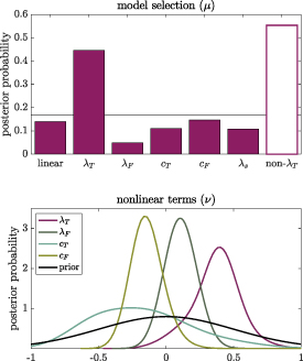
Figure 1. Top: posterior mass for the model selection parameter µ. Non-λT refers to all models other than the temperature-dependent feedback model. Bottom: posterior density for the nonlinear term ν in the four models with such a term.
Download figure:
Standard image High-resolution imageOther posteriors are relatively informative; the posteriors for the other nonlinear terms are not sign-definite, while the posteriors for c, τ, and λs
closely resemble their priors. One exception is that the lower-than-average time series of F are excluded from the posterior;  % of posterior probability is concentrated in ensemble members with an average of
  2.1 W m−2 over 1990–2020 (see figure S1 in SM), corresponding to greater than the 64th percentile of the F time series ensemble (i.e. prior). This is in agreement with the finding in [5] that the most negative prior aerosol forcing values were excluded from the posterior (figure 3 therein). Additionally, λ is fairly well-constrained to be on the upper end of its prior for models without a nonlinear feedback term, or close to the modal value for λ for those with a nonlinear feedback term (µ = 4 or 5; see figure S2 in SM). These together suggest that the historical T observations are more consistent with a high-radiative forcing and corresponding high-feedback parameter set.
Despite there being a clear preferred model structure, 55% of the posterior mass is in the remaining models, i.e.  . This strongly indicates an important role for structural uncertainty, especially given that the priors for the nonlinear terms in figure 1 are fairly broad, which is also the case for λs
. Figure 2 shows that indeed structural uncertainty is dominant for temperature projections under shared socioeconomic pathway SSP4-6.0; in this case
. This strongly indicates an important role for structural uncertainty, especially given that the priors for the nonlinear terms in figure 1 are fairly broad, which is also the case for λs
. Figure 2 shows that indeed structural uncertainty is dominant for temperature projections under shared socioeconomic pathway SSP4-6.0; in this case  and
and  , indicating that structural uncertainty is far larger than parametric uncertainty (u is our metric for the importance of structural uncertainty; see Materials and methods). This is even more pronounced for SSP3-7.0 (see figure S3 in SM), where
  and
and  . The multi-model median projection is also higher than the preferred-model-only projection; our focus here is on the uncertainty, however, especially given the discussion of the pattern effect above.
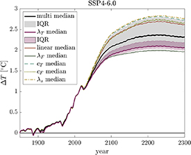
Figure 2. Projection of global mean surface temperature anomaly under the shared socioeconomic pathway SSP4-6.0. Lines denote the median projection of each model and of the multi-model ensemble. Purple (grey) shading denotes the interquartile range of projections for the temperature-dependent feedback model (multi-model ensemble).
Download figure:
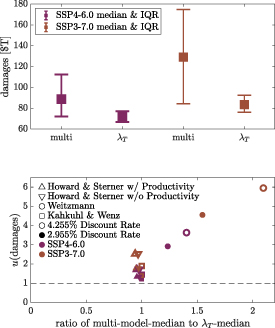
Standard image High-resolution imageThe primacy of structural uncertainty in temperature projections propagates into economic damages resulting from climate change as well. Figure 3 shows the interquartile range of damage calculations using the approach and default assumptions from [10] for SSP4-6.0 and SSP3-7.0. These assumptions include the damage function from Weitzman [25] and a discount rate of 4.255%, corresponding to a 1.5% pure rate of time preference, a global growth rate of 1.9%, and an elasticity of the marginal utility of consumption of 1.45. In both cases, the dominance of structural uncertainty is even more pronounced than in temperature; u for damages is 2.9 for SSP4-6.0, and 4.6 for SSP3-7.0. The importance of structural uncertainty holds for other discount rates and damage function assumptions; the bottom panel of figure 3 shows that the 'patient' discount rate of 2.955% from [10], corresponding to a pure rate of time preference of 0.1% rather than 1.5%, and/or alternate damage functions from [18] or [19] (the latter with or without changes to economic productivity) result in u > 1, i.e. greater economic uncertainty due to physical structural uncertainty than physical parametric uncertainty. However, the highest u values for damages occur for the Weitzman damage function used in [10], as do the discrepancies between the multi-model median and λT model median damages.
Figure 3. Top: median (squares) and interquartile range (error bars) of damages projected under the socioeconomic pathways SSP4-6.0 and SSP3-7.0 for the temperature-dependent feedback model and the multi-model ensemble, in trillions of 2019 USD. Damages are calculated over the period 2020–2300, with the default 4.255% discount rate and Weitzman damage function [25] from [10]. Bottom: u (i.e. ratio of structural vs. parametric uncertainty) for economic damages using different damage functions (shape), shared socioeconomic pathways (color), and discount rates (un/filled points), versus the corresponding ratio of median multi-model versus λT model damage estimates. u > 1 in all cases, as shown by the dashed black line for u = 1.
Download figure:
Standard image High-resolution image
These results demonstrate the importance of characterising structural uncertainty for physical and economic projections of climate. While we have focused on arguably the simplest representation of climate physics, even this single-equation energy-balance model is used in a variety of applications for which structural uncertainty has real physical and economic consequences. Our approach to characterising structural uncertainty is equally applicable to more complex representations of climate physics, such as the model used in [5]; if such a model is computationally efficient enough to generate an ensemble that captures parametric uncertainty, one can also use model selection parameters for its different components (e.g. a parameter choosing between several representations of the ocean circulation) in the same fashion. Doing so will be critical for robust uncertainty characterisation of these models. Even the most complex ESMs are subject to such structural uncertainty—possibly even more so as they involve so many parameterisations—though it is challenging to quantify either parametric or structural uncertainty, or the influence of internal variability, with such computationally expensive models.
Reductions in structural uncertainty may be possible by incorporating known phenomena such as the El Niño Southern Oscillation or the pattern effect more explicitly than we have done here, or leveraging other observations such as that of ocean heat content [26]. However, not accounting for temperature fluctuations due to climate oscillations can lead to overfitting, i.e. overconfidence in the 'preferred' model structure, because stochastic interannual and decadal natural climate variability unduly influences the inference of parameters like λ; the same goes for neglecting autocorrelation of residuals because the information content in a time-series is overestimated. Similarly, paleorecords provide a wider dynamic range of radiative forcing and temperature than the observational record, suggesting an opportunity to constrain structural uncertainty further. However, these temperature and radiative forcing changes are being continuously revised for even the most recent period used for such purposes, the Last Glacial Maximum [27]. Scientists tend to substantially underestimate uncertainty in these contexts [11] and model selection is very sensitive to such changes and what paleo-periods are considered (figures S4–S7). Paleo-observations either need to be used with a substantially inflated uncertainty and/or with extreme caution. We have also only considered a single nonlinear term at a time; it may also be fruitful to consider mixtures or combinations of these nonlinearities, or a nonlinear term that accounts for the pattern effect by having a λ term that first increases and then correspondingly decreases. In any case, we have shown here that structural uncertainty plays an important role in reduced complexity climate models' total uncertainty, which must be accounted for in their physical projections, and especially in the socioeconomic projections that use such simple representations of climate physics.
Acknowledgments
We thank the many scientists whose collective work has generated the time series, prior information, and statistical method on which our work relies. We also thank Chris Smith for providing the radiative forcing time series ensemble as well as insightful comments. Cael acknowledges support from the National Environmental Research Council through Enhancing Climate Observations, Models and Data. G L B acknowledges support from the Simons Foundation. D A S acknowledges support from the Grantham Research Institute on Climate Change and the Environment at the London School of Economics, the ESRC Centre for Climate Change Economics and Policy (CCCEP; Reference ES/R009708/1), and the Natural Environment Research Council through Optimising the Design of Ensembles to Syupport Science and Society (ODESSS; Reference NE/V011790/1).
Data availability statement
All data used here are publicly available at the sources cited in the text. Code is available at github.com/bbcael.
No new data were created or analysed in this study.
Author contributions
Cael lead all aspects of this work, with assistance from all other authors in methodology, interpretation, and writing.
Conflict of interest
The authors have no competing interests to declare.
Supplementary data (0.6 MB PDF)