

Abstract
The environmental fates and consequences of intensive sulfur (S) applications to croplands are largely unknown. In this study, we used S stable isotopes to identify and trace agricultural S from field-to-watershed scales, an initial and timely step toward constraining the modern S cycle. We conducted our research within the Napa River Watershed, California, US, where vineyards receive frequent fungicidal S sprays. We measured soil and surface water sulfate concentrations ([SO42−]) and stable isotopes (δ34S–SO42−), which we refer to in combination as the 'S fingerprint'. We compared samples collected from vineyards and surrounding forests/grasslands, which receive background atmospheric and geologic S sources. Vineyard δ34S–SO42− values were 9.9 ± 5.9‰ (median ± interquartile range), enriched by ∼10‰ relative to forests/grasslands (−0.28 ± 5.7‰). Vineyards also had roughly three-fold higher [SO42−] than forests/grasslands (13.6 and 5.0 mg SO42−–S l−1, respectively). Napa River δ34S–SO42− values, reflecting the watershed scale, were similar to those from vineyards (10.5 ± 7.0‰), despite vineyard agriculture constituting only ∼11% of the watershed area. Combined, our results provide important evidence that agricultural S is traceable at field-to-watershed scales, a critical step toward determining the consequences of agricultural alterations to the modern S cycle.
Export citation and abstract BibTeX RIS
1. Introduction
Crop sulfur (S) deficiency is increasing worldwide (McGrath and Zhao 1995, Feinberg et al 2021). Combined with climate change-driven changes in S-based pesticide demands (Caffarra et al 2012, Tang et al 2017), and widespread cropland intensification and expansion (Hu et al 2020), attention to agricultural S is growing (Scherer 2001, Hinckley et al 2020, Zak et al 2021). Changes to the global S cycle due to increased use of S applications in large-scale crop systems may have significant unintended consequences for ecosystem and human health, as well as affect the biogeochemical cycling of carbon, nitrogen, phosphorus, aluminum, and mercury (Hinckley et al 2020, Zak et al 2021). Thus, there is an emergent need to identify and trace agricultural S from fields and through watersheds to its ultimate fates.
Sulfur is ubiquitous in the environment, which confounds the detection and quantification of agricultural changes to the global S cycle. For example, some regions still experience elevated atmospheric S emissions (and deposition) from fossil fuel combustion (Klimont et al 2013), while others have substantial contributions from mineral weathering or mining S sources (Mitchell et al 2011, Zak et al 2021). However, for several decades, the stable isotopes of S, and principally the 34S/32S ratio, have provided a powerful tool to differentiate S sources and detect changes to the S cycle. Early studies of acid rain-impacted forests in Europe, the Northeastern US, and Canada used S stable isotopes to trace atmospheric S deposition into vegetation and soils (Case and Krouse 1980, Fuller et al 1986), to differentiate atmospheric from geologic S sources (Mitchell et al 1998, Mayer et al 2010), and to identify microbially-mediated processes affecting the timing and amounts of S exported to streams (Alewell and Gehre 1999, Novák et al 2005). Generally, microbial S transformations result in minimal S isotopic fractionation (Mitchell et al 1998), with the exception of microbial sulfate reduction (MSR), which strongly fractionates against 34S and is a predominantly anaerobic process (Kaplan and Rittenberg 1964, Bradley et al 2015). Thus, redox state is an important control on S transformations and S stable isotope ratios.
More recently, the utility of S stable isotopes has been expanded to a limited number of regional agricultural systems where S is applied intensively. The most comprehensive research has been in the Florida Everglades Agricultural Area. There, Bates et al (2002) used the S stable isotopes of sulfate (SO4 2−) to differentiate agricultural runoff from precipitation and groundwater S sources within downgradient wetlands. This approach linked agricultural S use in sugarcane farms to production of methylmercury (Orem et al 2011), a neurotoxin that bioaccumulates in fish and wildlife. Today, recent advancements in high-throughput, high-precision S stable isotope geochemistry (e.g. Mambelli et al 2016) create new opportunities to probe how agricultural S applications change the S cycle, particularly in systems beyond wetlands, which have unique biogeochemical cycling with predominantly reduced redox conditions.
In this study, we applied S stable isotopes to detect and trace agricultural S from field-to-watershed scales. We focused our research in California, US, where elemental S (S0) fungicide is the number one pesticide used Statewide, totaling ∼21 500 000 kg S per year (California Department of Pesticide Regulation 2020). We collected samples within the Napa River Watershed (figure 1). There, vineyard agriculture receives average cumulative applications of ∼80 kg S ha−1 yr−1—far exceeding the average annual atmospheric S deposition rate of 1.2 ± 0.5 kg S ha−1 yr−1 (Hinckley et al 2020). The Napa Watershed provides a natural contrast between the intensive vineyard agricultural S applications and surrounding hillsides of shrubland, grassland, and forests (henceforth 'non-agricultural areas') with background S sources (e.g. atmospheric and geologic).

Figure 1. Sampling locations. (a) The Napa River watershed land area consists of ∼11% vineyard agriculture, 63% forests, shrublands, and grasslands, and ∼15% suburban/urban development. We collected samples at 23 locations across the watershed (black labeled dots, see also supplementary table 1). (b) Sampling locations contrasted vineyard agriculture (top left), mixed forests (top right), and shrubland/grasslands (bottom).
Download figure:
Standard image High-resolution imageSpecifically, we tested: (a) S chemistry within and across vineyards with differing geology, topography, and S management practices; (b) differences between vineyard S chemistry and S chemistry in other source areas in the Watershed; and (c) whether vineyard S was detectable beyond fields. We collected soil leachate and surface water samples within multiple vineyard agriculture and non-agricultural areas, from Napa River tributaries, and in the mainstem of the Napa River over three years (figure 1; supplementary note; supplementary figure 1 available online at stacks.iop.org/ERL/17/054032/mmedia). We measured the S stable isotopic composition (34S/32S) of SO4 2− (δ34S–SO4 2−) and SO4 2− concentrations ([SO4 2−]), two measurements that, when combined, are widely used to characterize S sources and transformations (Bates et al 2002, Mayer et al 2010, Sambucci et al 2014). In this study, we define the bivariate combination of δ34S–SO4 2− and [SO4 2−] as an 'S fingerprint' and compare S fingerprints across land use types and from field-to-watershed scales.
2. Materials and methods
2.1. Study area
We measured δ34S–SO4 2− and [SO4 2−] in soil leachate and surface water samples collected throughout the Napa River Watershed, California, US. This watershed is 1103 km2 and is dominated by two contrasting land use/land covers (LULCs): wine grapes are grown nearly exclusively throughout the Napa Valley (∼11% of the watershed area) and are surrounded by hillsides of forests (26%) and woodlands (37%; figure 1). The Watershed encompasses the traditional and contemporary territories of the Lake Miwok, Coast Miwok, Southern Pomo, Wappo, and Patwin peoples. The Napa River drains into extensive wetlands in San Pablo Bay, connecting to the greater San Francisco Bay Estuary.
The region's Mediterranean climate strongly influences seasonal hydrology and agricultural management practices. Wine grapes grow during the dry season (April through September) and farm workers spray elemental S (S0) fungicide weekly to biweekly to prevent powdery mildew infection. Tributaries to the Napa River are largely dry during this period. During the wet and dormant crop season (October through March), nearly all annual precipitation falls as rain. There is a gradient in precipitation from north to south in the watershed: 931 mm in St. Helena to 518 mm in Napa (Arguez et al 2012). Rains periodically saturate vineyard soils to ⩾0.5 m depth, mobilizing S below the vine rooting zone and affecting soil porewater δ34S–SO4 2− values (Hinckley et al 2008, Hinckley and Matson 2011). Rains also activate tributary flows. Although redox profiles were not collected in this study, observations of surface water ponding throughout wet seasons suggests the potential for dynamic redox conditions in vineyard soils.
2.2. Soil leachate and surface water sampling
We established sampling locations within the predominant LULCs in the watershed and to incorporate the precipitation gradient and variability in underlying geologies (figure 1; supplementary table 1). We collected samples during 11 field campaigns, focusing efforts during the wet seasons of water years 2018–2020 (supplementary figure 1).
We sampled soil leachate from six vineyards, one forested area, and one grassland area. At each sampling site, we installed four tension lysimeters (SoilMoisture, Inc.) across one vineyard management block or equivalent area (for the non-vineyard sites; ∼1–2 ha) to capture spatial heterogeneity. Lysimeters were installed to 0.5–0.6 m depth, except at four steep sites, where lysimeter depths targeted shallow (0.2–0.3 m) and deep (0.4–0.6 m) flow paths. We purged lysimeters once before collecting samples into polycarbonate VacLok 60 ml syringes (Merit Medical Systems) or high density polyethylene bottles under vacuum. The lysimeters did not appear to affect δ34S–SO4 2− values (supplementary figure 2).
We also collected water samples from rain, irrigation lines, culvert outflows, tributaries, and the Napa River. We pre-rinsed HDPE bottles three times with sample water before filling completely to minimize headspace. Rainwater was collected into aluminum trays pre-rinsed with deionized water. We filtered all water samples through sequential 0.8 µm (Pall Acrodisc, sterile Supor polyethersulfone) and 0.45 µm (VWR, sterile polyethersulfone) 25 or 47 mm filters, stored and shipped samples on ice, and then we froze samples (∼−20 °C) until processing and analyses. We analyzed six S0 fungicide samples provided by winegrower collaborators.
2.3. Laboratory analyses
We analyzed samples for [SO4 2−] and the S stable isotope composition of SO4 2− or S0. We measured [SO4 2−] using an ion chromatograph (Dionex; detection limit 0.2 mg S l−1, relative percent difference between sample duplicates ⩽5%). To prepare aqueous samples for S stable isotope analysis, we thawed samples overnight and then precipitated BaSO4 (Hinckley et al 2008). Briefly, we acidified samples to within a pH of 2–4 with hydrochloric acid (Fisher Chemical, trace-metal grade), brought samples to a boil, and added 10% (w/w) BaCl2 solution (MilliporeSigma, ACS grade) in excess. We collected BaSO4 precipitate on 0.45 µm Whatman mixed cellulose ester filters, which we then dried overnight at 60 °C. We analyzed solid BaSO4 and S0 samples for δ34S on a Flash IRMS elemental analyzer coupled with a Delta V Plus isotope ratio mass spectrometer (Thermo Fisher Scientific EA IsoLink). We report stable isotope values in conventional δ-notation in parts per 1000 (‰; Sharp 2017) and relative to the international standard Vienna-Canyon Diablo Troilite. Long-term analytical precision for isotope analysis is ±0.2‰ based on using internal reference standards calibrated annually against International Atomic Energy Agency-certified reference materials.
2.4. Statistical analyses
Statistical analyses were conducted in R software (v.4.0.4; R Core Team 2021). We selected non-parametric analyses, because the data violated the parametric assumptions of normality and sample independence. We tested the null hypothesis that median δ34S–SO4 2− values and [SO4 2−] were equal across LULC groups using a non-parametric Kruskal–Wallis test (Kruskal and Wallis 1952), followed by post-hoc Dunn's test (Dunn 1964) with a Holm's p-adjustment (Holm 1979). We chose a p-value < 0.05 to determine statistical significance and, throughout, values are reported as the median ± interquartile range.
3. Results and discussion
3.1. Patterns of agricultural and non-agricultural S fingerprints from field-to-watershed scales
Despite differences in the quantity of S applied, underlying geology, regional climatology, and topography (supplementary table 1), the six vineyards sampled followed a general pattern showing an increase in median δ34S–SO4 2− values from lower to higher S concentrations (figure 2; Hermes and Hinckley, 2021). Vineyard δ34S–SO4 2− values were 7.2 ± 5.2‰ below 22 mg SO4 2−–S l−1 (n = 35; range = 13.7‰) and shifted to 12.8 ± 3.7‰ (n = 20, range = 11.5‰) above 22 mg SO4 2−–S l−1. We compared our measurements to prior data collected intensively in an additional vineyard (Hinckley et al 2008) and found that the overall pattern was remarkably consistent, suggesting that the vineyard S fingerprint is detectable within and across vineyards and over time (supplementary figure 2).
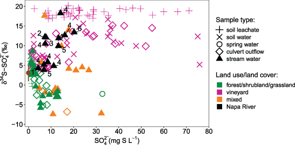
Figure 2. Sulfur fingerprints. Vineyard agriculture S fingerprints compared to non-agricultural areas (primarily forest, shrubland, and grassland) and mixed LULC tributaries. Numbers indicate Napa River transect samples from headwaters (1) to just above the tidal extent (6) with repeat sampling conducted at transect site number 4 (supplementary table 1). Sulfur sources include S fungicide (brown bar representing mean and range, n = 6) and irrigation and precipitation water from Hinckley et al (2008; gray shaded box). Soil leachate data designated as '+' symbols are laboratory-based measurements from one vineyard and represent soil-only measurements without the influence of mixing with irrigation and precipitation water (Hermes et al 2021).
Download figure:
Standard image High-resolution imageThe S patterns from vineyard agriculture and non-agricultural areas of the watershed were strikingly different (figure 2). Non-agricultural soil leachate and surface water had δ34S–SO4 2− values of −0.28 ± 5.7‰ (n = 30, range = 14.4‰), depleted by ∼10‰ relative to vineyards (9.9 ± 5.9‰; n = 55, p = 1.2 × 10⁻¹⁰). Surface waters from non-agricultural areas also had roughly three-fold lower [SO4 2−] than vineyard samples (5.0 ± 5.5 and 13.6 ± 26.6 mg SO4 2−–S l−1, respectively; p = 1.1 × 10⁻⁴), although we note that a number of vineyard waters had similar [SO4 2−] to those from non-agricultural areas (∼1–15 mg SO4 2−–S l−1, n = 29, figure 2). Within individual sub-catchments, vineyard agriculture δ34S–SO4 2− values were enriched by 17.8–20.5‰ relative to adjacent non-agricultural areas (supplementary figure 3). Our results clearly indicate that vineyard agriculture has a consistent S biogeochemical fingerprint that is distinct from non-agricultural areas.
Moving beyond agricultural source areas (fields), culvert outflows and tributaries to the mainstem of the Napa River reflected a combination of vineyard and non-agricultural sources. We found that vineyard culvert outflows had δ34S–SO4 2− values and [SO4 2−] similar to soil leachate (figure 2), suggesting that the S fingerprint found in vineyard soil leachate is carried by drainage outflows into the broader watershed. Tributaries draining mixed LULC areas had δ34S–SO4 2− values that spanned the entire range measured, from −7.4 to 17.6‰, and [SO4 2−] of 13.0 ± 7.1 mg SO4 2−–S l−1 (n = 17), which were intermediate to vineyard agriculture and non-agricultural endmembers. Two tributaries with 12% and 23% vineyard land cover, respectively, had δ34S–SO4 2− values (∼4–18‰) that were more similar to vineyard soil leachate and surface waters than the predominant non-agricultural areas in those sub-catchments (supplementary table 1). However, it is worth noting that their δ34S–SO4 2− values changed from ∼4–6‰ to 10–18‰ between early-season and late-season sampling campaigns (supplementary figure 3). We hypothesize that these changes in δ34S–SO4 2− values reflect within-season shifts in the contributions of vineyard and non-agricultural S sources depending on source area hydrologic activation and connectivity to tributary channels. Overall, our ability to detect the influence of the vineyard S fingerprint within tributaries indicates that vineyard S is detectable at sub-watershed scales.
To capture the watershed scale, we measured S fingerprints in surface water from the mainstem of the Napa River, which fell within the range of vineyard measurements (p = 0.9) and varied spatially and temporally. Napa River samples had δ34S–SO4 2− values of 10.5 ± 7.0‰ and 8.5 ± 6.1 mg SO4 2−–S l−1 (n = 13; figure 2). To examine spatial changes to the S fingerprint along the Napa River, we sampled a transect from the headwaters to just below the tidal extent (figure 1(a); supplementary table 1). The headwaters drain non-agricultural (primarily forested) areas and had similar S chemistry to that of non-agricultural tributaries (4.3‰ and 4.3 mg SO4 2−–S l−1; point 1, figure 2). Moving downstream, transect samples increased in [SO4 2−] and δ34S–SO4 2−, consistent with the increase from 0% to 5%–15% vineyard agriculture in contributing areas (points 2–6, figure 2; supplementary table 1). Overall, transect samples had δ34S–SO4 2− values of 4.3–13.4‰ and 4.3–20.2 mg SO4 2−–S l−1. We captured temporal variability through repeat sampling of the Napa River above the city of Napa, CA and found that δ34S–SO4 2− values ranged from 4.9 to 18.3‰ with 6.9–16.1 mg SO4 2−–S l−1 (n = 7; figure 1(a); point 4, figure 2). These results show that the Napa River S fingerprint varies temporally by as much as it does spatially along the transect (figure 2). Similar to the shifts in S chemistry observed in tributaries, we suggest that the shift in δ34S–SO4 2− and [SO4 2−] at the repeat sampling location could arise from changes in source water contributions over the course of the wet season. Linking hydrology and S chemistry at catchment-to-watershed scales is an outstanding, but critical, research direction. Nevertheless, the overall enriched S stable isotope signal and elevated [SO4 2−] within the Napa River indicate that the vineyard S fingerprint remains predominant at the watershed scale.
3.2. Examining S sources and processes
The notable contrast between S stable isotope values derived from vineyard and non-agricultural areas yields insights into S sources and dominant processes within fields and sub-catchments. To examine S sources, we compared laboratory-based grassland (non-agricultural) and vineyard soil leachates (Hermes et al 2021) to S inputs (figure 2). Soil leachate δ34S–SO4 2− values in non-agricultural areas were 4.9 ± 5.0‰ (n = 14), similar to precipitation water (5.5‰; n = 1; Hinckley et al 2008) and surface waters from non-agricultural areas (−0.3 ± 5.7‰; n = 27). The isotopically-depleted soil leachate, culvert, and stream water in non-agricultural areas likely reflect a mixture of precipitation and geologic S sources enriched in 32S, as occurs with the oxidation of reduced S species from geologic weathering or springs (Grasby et al 1997, Mayer et al 2010). In contrast, repeated laboratory-based measurements of soil leachate from one vineyard had δ34S–SO4 2− values (n = 38) that were enriched by ∼15.3‰ relative to S fungicide (3.1 ± 1.8‰, n = 6) and by ∼13‰ relative to irrigation and precipitation water (5.7 ± 0.5‰; n = 10; figure 2). Field-based vineyard soil leachate δ34S–SO4 2− values fell in between the laboratory leachates and S sources—similar to the mixing of soil waters and sources reported by Hinckley et al (2008). Although the enriched vineyard soil leachate δ34S–SO4 2− values could reflect additional S sources to vineyards such as gypsum—a soil conditioner—not all vineyards we sampled apply gypsum (supplementary figure 4). Rather, the discrepancy between soil leachate δ34S–SO4 2− and S sources in vineyards implies that additional S fractionation processes occur.
We hypothesize that a number of microbially-mediated S transformations that fractionate S within soils may affect the isotopically enriched vineyard S fingerprint, as summarized in a conceptual model (figure 3). Within vineyards, rapid oxidation of S0 fungicide following application to soils during the dry, growing season results in accumulation of SO4 2− and immobilization into organic S species (Germida and Janzen 1993, Yang et al 2010, Hinckley et al 2011), both processes with minimal S stable isotope fractionation (Mitchell et al 1998, Chalk et al 2017). We hypothesize that the enriched vineyard soil leachate δ34S–SO4 2− values relative to S inputs could be derived from MSR, a process that strongly fractionates 34S/32S and enriches the residual SO4 2− pool (Kaplan and Rittenberg 1964, Bradley et al 2015). Although typically found in low oxygen environments (Barton and Fauque 2009), MSR could occur during intermittent-to-sustained soil saturation during irrigation events, the wet season, and/or in soil anoxic microsites within oxygenated soils (Hansel et al 2008, Santana et al 2021), similar to the discovery that oxic soils host high rates of methanogenesis (Angle et al 2017). Since sulfur isotope fractionation is inversely related to sulfate reduction rate (Kaplan and Rittenberg 1964), even slow rates of MSR could impart a strong effect on vineyard soil δ34S–SO4 2− values. In contrast to S biogeochemistry within vineyards, depleted δ34S–SO4 2− values in forested/grassland areas compared to vineyards likely reflect mixing of atmospheric and geologic S, enriched in 32S (Mayer et al 2010). We next discuss additional processes that may prevent 'runaway' enrichment of the soil SO4 2− pool within vineyards.
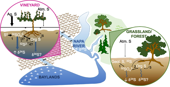
Figure 3. Conceptual model. A conceptual model of S biogeochemical cycling in vineyard agriculture vs non-agricultural areas of the Napa River watershed. Sulfur is sprayed on vineyards ('Ag. S') at cumulative average rates ∼16–20 times higher than atmospheric deposition ('Atm. S'). Ag. S additions stimulate microbial S oxidation (1) and subsequent immobilization of SO4 2− into organic S ('Org S'; (2)), transformations with minimal S isotope fractionation. We hypothesize that microbial S reduction (3) is stimulated within vineyard soils, which strongly fractionates between 34S/32S and results in the enriched SO4 2− pool that we measured in vineyard soil and stream surface waters. Sulfide incorporation into the organic S pool (4) and recycling between organic and inorganic S species remain important but understudied aspects of the S cycle (denoted by question marks). At broader spatial scales, irrigation, tile drains, terraces, and other water management strategies within vineyards (black pipes, linear flow paths) influence soil water storage and redox conditions and water and S export to tributaries and the Napa River. In contrast, forested/grassland areas are predominated by atmospheric S, geologic S enriched in 32S ('Geol. S'), and organic matter decomposition (5) with largely unmodified hydrologic flow paths, resulting in depleted δ34S–SO4 2− values relative to vineyards. At the watershed scale, the Napa River has enriched δ34S–SO4 2− values, suggesting that vineyard agricultural S is the predominant source.
Download figure:
Standard image High-resolution imageWe hypothesize that three additional processes may act to constrain the agricultural S fingerprint. First, there has been little research into how soil wetting and drying cycles control the balance of S oxidation and reduction during irrigation events or the wet season. Sulfur oxidation can result in ∼1‰ depletion of the SO4 2− pool (Wainwright 1984); this process could act to counter the enrichment effects of MSR on δ34S–SO4 2− values (figure 3). Highly managed irrigation practices and water routing through tile drains and ditches within and surrounding vineyards likely influence soil redox state as well as S transport to streams by controlling water residence times. Alternatively, although sulfide produced by MSR is rarely measured or studied in upland agricultural soils (Wainwright 1984), if it is indeed produced, it could be abiotically scavenged by the predominant organic S pool (Sleighter et al 2014, Poulin et al 2017). Upon organic S remineralization, the newly formed SO4 2− would carry the depleted 34S signature from MSR, limiting further enrichment of δ34S–SO4 2− values. Secondary SO4 2− production from organic S remineralization is an additional source of SO4 2− in forested ecosystems (Mayer et al 1995, Marty et al 2019), and more research is needed to understand the effects of cycling between organic and inorganic S on δ34S–SO4 2− values and [SO4 2−]. Finally, reactive S intermediate species may complicate studying agricultural S transformations within soils, known as the 'cryptic' S cycle (Hansel et al 2015). A key next step in examining the S cascade is to conduct studies that constrain the enriched, asymptotic agricultural S fingerprint, including measurements of soil redox conditions alongside S biogeochemical processes and rates and S-isotope fingerprinting.
3.3. Putting the Napa River Watershed into a global context
To put our measurements from the Napa River Watershed into perspective, we compared our δ34S–SO4 2− values and [SO4 2−] to those from rivers around the world, compiled by Burke et al (2018). Our δ34S–SO4 2− measurements collected throughout the Napa River Watershed were strikingly similar to the pattern of values from rivers (figure 4). Burke et al (2018) calculated a modern flux-weighted global riverine δ34S value of 4.4 ± 4.5‰ (1 s.d.). Our overall average δ34S–SO4 2− value of 6.13‰ was slightly enriched from this mean, but within one standard deviation. Globally, river δ34S–SO4 2− values ranged from −13.4 to 21.7‰, and, remarkably, our samples from within the Napa River Watershed alone accounted for much of this variability (−7.4–18.3‰). The spatial and temporal variability we found along the Napa River is similar to Burke et al's (2018) note that δ34S values from a single river can range widely, driven by varying tributary contributions with different S sources (Burke et al 2018).

Figure 4. Comparison to river δ34S values from around the world. Data from this study (depicted as in figure 2) compared to data from Burke et al (2018; black dots). The gray dashed line indicates the modern flux-weighted global riverine average δ34S value (Burke et al 2018). Note the log scale on the x-axis.
Download figure:
Standard image High-resolution image
Comparing our measurements to the global dataset (Burke et al 2018) also reinforced the importance of considering both S sources and processes in interpreting δ34S–SO4 2− values. The lowest global δ34S–SO4 2− values measured (−8.5 to −13.4‰) were from the Santa Clara River in Southern California—reflecting oxidation of pyrite and organic S from organic-rich shales and sandstones of the Monterey Formation. Some of our depleted δ34S–SO4 2− values from non-agricultural tributaries drain the Great Valley Complex, a similar shale/sandstone bedrock. However, our non-agricultural values may be less depleted than the Santa Clara River overall due to the highly heterogeneous geology of the Napa Watershed. The highest global δ34S–SO4 2− values measured (∼14–22‰) were from the Lena and Yenisei rivers draining the Siberian Platform, a source of enriched evaporite S. While evaporite S as an additional agricultural input to vineyards could contribute to our enriched S values, it could not fully explain the pattern we observed across multiple vineyards (supplementary figure 4), further reinforcing that MSR could account for additional enrichment. Changes to δ34S–SO4 2− values from MSR could result in an overestimation of evaporite S contributions to the global S cycle if MSR affects δ34S values more broadly. Overall, comparing our measurements to global values reinforces that intensive agricultural S additions can significantly alter the δ34S–SO4 2− signature of tributaries and rivers, affecting S source flux attributions and revealing the importance of delving into microbial dynamics when interpreting the global river δ34S pattern.
3.4. Implications for S fates, consequences, and management
This study provides the first evidence that intensive agricultural S applications change the biogeochemical fingerprint of S at field-to-watershed scales in an upland, mixed LULC watershed. The dramatic difference between δ34S–SO4 2− values from vineyard agriculture and non-agricultural areas (9.9 ± 5.9‰, n = 55, vs −0.28 ± 5.7‰, n = 30, respectively; figure 2) provides clear and compelling evidence for an altered S cycle in agricultural areas. Furthermore, the persistence of the agricultural S fingerprint in the Napa River—very similar to that found in soil leachate from fields—suggests that intensive S applications alter the S cycle at watershed scales, despite their input to a minor proportion of the watershed area. Ultimately, this study demonstrates the potential to understand the modern S cascade in agricultural systems, which is critical to documenting and developing solutions to human manipulation of the S cycle more broadly.
Acknowledgments
We thank M Cooper, cooperating vineyard managers and landowners, Napa County Resource Conservation District, and the Napa County Regional Park and Open Space District for site access, as well as S Mambelli and W Yang for assistance with sample analyses. This research was funded by a National Science Foundation RAPID Award (EAR-1808034) and NSF CAREER (EAR-1945388) to E-L S Hinckley, and a Geological Society of America Graduate Student Research grant and National Geographic Early Career award to A Hermes.
Data availability statement
The data that support the findings of this study are openly available at the following URL/DOI: https://doi.org/10.6073/pasta/8b81b39d87d5f70325420294ffc83ddf.