

Abstract
Plastic pollution is a critical environmental concern. There is a growing focus on this transboundary issue, and a corresponding increase in public and government awareness. Understanding the key factors associated with litter and mismanaged waste on land will help to predict where and how waste enters the environment, providing opportunities for low cost, effective interventions. There exist only a few large-scale datasets with which such analyses can be conducted. To fill this knowledge gap we analysed a national, designed survey dataset of litter in the environment from Keep Australia Beautiful (2007–2017). We found that debris decreased significantly, with a nearly 6% decrease over the decade. Using generalised additive model modelling of 17 653 surveys at 983 sites around Australia, we found that site type, land use, state, population, and socio-economic status had the strongest relationships (in decreasing order) with litter distribution. Higher levels of litter were found in economically and socially disadvantaged neighbourhoods. Site types related to transitory human use such as highways and carparks, had more litter than areas with higher aesthetic or cultural value such as beaches, parks, and residential neighbourhoods. Sites that were sources of litter, such as shopping centres and retail strips, also had elevated litter counts, as did surveys near waterways. This enhanced understanding of the factors that influence litter deposition will help to craft more effective policy solutions, and can also improve our models of litter loads on land, and subsequent input to the ocean.
Export citation and abstract BibTeX RIS

Original content from this work may be used under the terms of the Creative Commons Attribution 4.0 license. Any further distribution of this work must maintain attribution to the author(s) and the title of the work, journal citation and DOI.
1. Introduction
Marine plastic pollution has rapidly become one of the pressing environmental concerns of the 21st century. Because of its adverse impacts on wildlife, human health, and the economy, it has been identified as one of the main targets within the UN's sustainable development goals (SDGs) (UN General Assembly 2015). One target of SDG 14 is to 'reduce marine pollution of all kinds, particularly from land-based activities.' Approximately 80% of marine plastic pollution is thought to originate from mismanaged waste on land (Derraik 2002). Global modelling suggests that between 19 and 23 million tonnes of debris enter aquatic ecosystems annually (Borrelle et al 2020). In Australia, it has been estimated that there are more than 120 million pieces of debris around the country's coastline (Hardesty et al 2017).
To determine where to best implement interventions to reduce waste leakage and evaluate which of the myriad of available approaches will work most effectively, it is useful to understand the underlying drivers of mismanaged waste. Typically, estimations of mismanaged plastic waste rely heavily on local population density (e.g. Jambeck et al 2015, Lebreton and Andrady 2019). However, there are many other factors which could potentially influence the distribution of litter, including socio-economic status (SES) (Matsunaga and Themelis 2002), environmental variables such land cover (Sakti et al 2021), and waste and transport infrastructure (Willis et al 2017).
While there is a growing body of literature that has quantified the economic impacts of litter (Jang et al 2014, Leggett et al 2018, Newman et al 2015, Watkins and ten Brink 2017), our knowledge about the role of SES as a driver of this litter is relatively sparse. Hardesty et al (2021) analysed debris across 118 different countries and reported that debris was negatively correlated with national wealth, and positively with the value of infrastructure in the local area (Hardesty et al 2021). A few publications discuss the relationship between self-reported attitudes about littering and education or economic status (Santos et al 2005, Widmer and Reis 2010, Slavin et al 2012, Eastman et al 2013). Most conclude that higher levels of education or income correlate with a decreased propensity for littering (but see Arafat et al 2007). Similarly, while there have been attempts to correlate physical forcing factors with debris distribution on beaches and on the sea floor (Thornton and Jackson 1998, Galgani et al 2000, Ribic et al 2010, 2011, 2012), few have investigated the effects of environmental factors on the distribution of litter in the inland terrestrial environment.
To address this knowledge gap and help identify where to best target interventions to reduce waste leakage from land, we analysed data from urban areas around Australia. We asked whether environmental and social factors can explain the distribution of litter in the terrestrial environment at a national scale. We considered four indices of SES (economic advantage, economic disadvantage, economic resource, and education and occupation), as well as measures of infrastructure (roads, rail networks, and landfills), population density, land use, site type, and time (years since 2007).
2. Methods
2.1. Debris data
We compiled data gathered by Keep South Australia (SA) Beautiful and Keep Australia Beautiful (hereafter referred to as KAB) from 2007 to 2017 as part of the National Litter Index (NLI). The NLI is conducted bi-annually at a set of fixed locations in cities around Australia (figure 1). Survey locations are distributed across a variety of site types defined by KAB (beaches, car parking areas, recreational parks, residential areas, roadside retail strips, shopping centres, highways, and industrial zones). The site locations remain constant from year to year, except in rare instances where the site usage changes (e.g. from residential to industrial) or where landform changes make it impossible to re-survey the same area. Locations are kept anonymous to ensure an unbiased sample from year to year.

Figure 1. Debris counts (Items/1000 m2) for each study across all years of KAB data (2007–2016), in each state of Australia (South Australia (SA), Western Australia (WA), Northern Territory (NT), Queensland (QLD), New South Wales (NSW), Australian Capital Territory (ACT), Tasmania (TAS), and Victoria (VIC)). Red colours indicate higher counts of debris. Purple circles indicate outlier sites of over 2000 items/1000 m2 (ten sites in total).
Download figure:
Standard image High-resolution imageAt each location, trained observers count and classify all of the litter that they see within the specified survey area. Surveyed areas range in size between 71 to 9600 m2, with an average of 1526 m2. In the annual NLI reports (Keep Australia Beautiful 2019), results are reported as the number of items/1000 m2, so we have used this convention for comparability.
2.2. Driving variables (covariates)
For each survey site, we estimated the geospatial position based on written and photographic information provided by KAB. We used this position to compile data on each of the different factors that might affect debris loads (covariates). These included the distance from each site to the nearest road (Geoscience Australia 2006), rail station (Geoscience Australia 2006), and landfill (Department of the Environment and Energy 2018), and the land use at each survey site (Australian Bureau of Agricultural and Resource Economics and Sciences (ABARES) 2016). Within a 1 km, 5 km, and 50 km radius, we calculated the total population (Australian Bureau of Statistics 2016), total length of roads (Geoscience Australia 2006), and the average values of four different socio-economic indices (economic advantage, economic disadvantage, economic resource, and education and occupation) based on census data from the Australian Bureau of Statistics (Australian Bureau of Statistics 2011). The four different indices each highlight slightly different aspects of the SES of an area (table 1), and all are strongly correlated. We therefore could only include one index as a main effect, but we were interested in the information provided by the other variables. Therefore we calculated the residuals of linear regression models between the main effect index and each of the other indices (See SI available online at stacks.iop.org/ERL/17/045013/mmedia).
Table 1. Description of all of the covariates that were assessed in the modelling. Note that all of the numeric variables were scaled in order to better compare effect sizes between categorical and numeric variables (Gelman 2008). Range of original values are reported for numeric covariates that appear in the best-fit model.
| Category | Variable | Units/range | Description |
|---|---|---|---|
| Socio-economic indices (2011) | Index of Relative Socio-Economic Advantage and Disadvantage (IRSAD) | Score incorporates measures of advantage (e.g. high income, mortgage, diploma, cars ownership, etc). Higher values indicate lack of disadvantage and greater advantage generally | |
| Index of Relative Socio-Economic Disadvantage (IRSD) | R: (707–1132) | Relative measures of disadvantage (low English speaking, income, qualifications, low skill occupations, etc). Higher values indicate less disadvantage | |
| Index of Education and Occupation (IEO) | Includes measures of occupation and education. High score indicates higher education and occupation status | ||
| Index of Economic Resources (IER) | Only includes financial aspects of socio-economic status. High score indicates greater access to economic resources. | ||
| Residuals value of Advantage/Disadvantage | Residuals of a linear model relating IRSAD to IRSD | ||
| Residuals value of Education/Disadvantage | R: (−104.24–179.65) | Residuals of a linear model relating IEO to IRSD | |
| Residuals value of Resource/Disadvantage | Residuals of a linear model relating IER to IRSD | ||
| Population density | Log of population at 5 km radius and 50 km radius | R: (3.29–12.74) R: (9.52–15.29) | Log of total population figures within a 5 and 50 km radius as at 2014 from Australian Census |
| Population Residuals (5 km to 50 km) | R: (−1.4 E05–1.8 E05) | Residuals of a linear model relating total population within 5 and 50 km radius | |
| Population at 1,5, and 50 km radius | Total census population as at 2014 | ||
| Infrastructure | Total length of roads (within 1 km radius) | Kilometers R: (0–12.8) | Total length of roads |
| Road residuals (5 km to 50 km radius) | Continuous variable R: (−64.6–87.1) | Residuals of a linear model relating total length of roads within 5 and 50 km radius | |
| Dist to nearest rail station | Kilometres R: (0.02–64.65) | Distance to nearest rail station | |
| Dist to nearest landfill | Kilometres R: (0.03–26.81) | Distance to nearest landfill | |
| Dist to nearest road | Kilometers | Distance to the nearest road | |
| Sampling variables | Relative site area surveyed | R: (1–161.98) | Size of the area for each survey, relative to the smallest site |
| Time Trend | Year | R: (1–11) | Number of years from start of survey in 2007 |
| Year*State | Interaction term | Interaction term between state and time trend | |
| State | State | Categorical—7 levels | Each of the seven Australian states and territories |
| Landuse | Landuse | 6 categories | Catchment-scale landuse |
| Site Type | Site type | 8 categories | As defined by KAB |
We wanted to know if there is a discernible difference between local and regional population density and infrastructure, and debris counts at NLI survey sites. Regional population (total population within a 50 km radius) is highly correlated with local population density (total population within a 5 km radius), so we calculated the residuals of a linear model between population within a 5 km radius vs. population in a 50 km radius, and roads within a 5 km radius vs roads within a 50 km radius. We included these residuals as predictors in the model, allowing us to separate out the local and regional effects of road and population density. We also tested the potential for a non-linear relationship between population density and debris by incorporating the log of the population density at 5 and 50 km.
To provide more detail around the question of time trends, we added an interaction term between Year and State.
2.3. Statistical analyses
To compare the relative effect sizes between both numeric and categorical variables, and to make the fit more stable, we scaled all of the numeric variables before fitting. We subtracted the means and divided by twice the standard deviations (Gelman 2008). This allows for a more direct comparison of coefficients between variables with different means. The higher the absolute value of the coefficient, the more influence that factor has on the debris density.
We used the total number of items found on each survey as the response variable, and fit an offset term for the total square metres surveyed. We were concerned that differences in the total area surveyed at each site could affect the search effort, so we accounted for this potential variability by including a term for the relative area surveyed as a predictor in the model.
We fit generalised additive models (GAMs) to the data using the R program and mgcv and MuMin packages (Bartoń 2018, Wood 2011, R Core Team 2018). We chose the GAM package because it accommodates the Tweedie distribution, but we used parametric terms in the model in order to be able to make predictions outside of our study sites. We restricted the models from incorporating any main effect terms with a correlation coefficient stronger than 0.6, and used MuMin's dredge function to find the combination of predictor variables that yielded the lowest Akaike information criteria (AIC). AIC is a measure which balances parsimony and fit, where the lowest value indicates the best-fit model (Burnham and Anderson 2002). After finding the best model for the main effects, we tested whether adding the residual values for the remaining socio-economic indices would improve the AIC value, and chose the one that reduced it the most (see SI for more details).
Finally, we calculated the percent decrease in total debris found over time. We created a dummy dataset and set all of the variables to a constant, with the exception of Year. For the numeric variables we used the median value of the original data set, and for the categorical variables we used the most frequent value in the data set. We then predicted the debris levels using the final model, and calculated the percent change over time.
3. Results
A total of 983 sites were sampled over the 11 year period, with the vast majority of the sites (946) being sampled either 18 (n = 946) or 17 (n = 20) times.
The best-fit GAM model (lowest AIC value) included a number of socio-economic and infrastructure factors (table S1, figure 2). The coefficients for all terms were significantly different from zero, except for road distance, population residuals, and several of the state terms. Leaving any of these terms out increased the AIC, indicating that these terms, although some were not significantly different from zero at a p < 0.05 level, still made an important contribution to the fit of the model. The deviance explained by the model was 32.5%, meaning that the model explained over 32% of the variability in the data.

Figure 2. Standardised effect sizes for the best fit GAM model. Positive values (triangles) indicate a positive correlation with total debris loads, while negative values (circles) indicate a negative correlation. Note that for each factor, the values for a reference level are captured within the intercept term, and the remaining terms are considered with respect to the reference level. Reference levels for this model include (State: ACT, Site Type: Beach, Land Use: Conservation). The colours show the significance levels (p-values).
Download figure:
Standard image High-resolution imageFor the continuous variables, relative area was the strongest predictor of debris load. Aside from this artefact of the sample design, the next strongest predictors of debris load were the log of the population density within 5 km, the index of economic disadvantage, and the survey year. The index of economic disadvantage measures not only the economic status of individuals, but more broadly measures their 'access to material and social resources, and their ability to participate in society' (Australian Bureau of Statistics 2011). A lower score on this index indicates greater disadvantage, and a higher score indicates a lack of disadvantage (though not necessarily advantage). The higher the index of economic disadvantage, the less litter reported.
We also measured three different socio-economic residuals, to understand the relative influence of education, resources (more narrowly defined as access to economic resources), and advantage (incorporates not only measures of disadvantage, but also economic and social indicators of advantage). Only one, the residual value between education and disadvantage, was significant, and improved the model. This residual was positively correlated with debris levels, meaning that higher-than-expected education indicators at a given level of social disadvantage was correlated with higher levels of debris. Similarly, the residual for advantage/disadvantage was positive (though not significant at the p < 0.5 level), while the residual for resource/disadvantage yielded a negative correlation, though was also not significant at the p < 0.5 level.
For the categorical variables, the strongest predictors of litter were site type and land use. Highways and retail strips had elevated levels of litter relative to other site types (figure 3). In contrast, recreational parks, residential areas, and beaches were relatively low. Land use was also important in determining loads. Areas classified as 'water' (including creeks and wetlands), had the highest debris loads, followed closely by 'production from the natural environment', which is land used for primary production where there is little change to the native vegetation (Australian Bureau of Agricultural and Resource Economics and Sciences (ABARES) 2016).
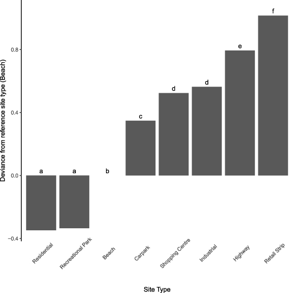
Figure 3. Comparison of the model coefficients for each of the site types, relative to the reference (Beach). Site types with the same letter do not differ significantly from one another, those with different letters are significantly different (p < 0.05)
Download figure:
Standard image High-resolution imageA number of measures of urbanization are relevant for litter loads. Population density within 5 km was positively correlated with litter (on a log scale), while population density within 50 km was negatively correlated (also log scale). Litter levels are higher near rail stations and closer to roads (though this measure was not significant). Sites with a lower road density surrounded by regions with higher density of roads have higher levels of debris. Additionally, litter levels were higher closer to waste management facilities. However, these factors (other than population density within 5 km) have relatively low effect sizes, suggesting they are less important than socio-economic variables, land use, and site type.
Even taking into account the variability captured by the other terms in the model (site type, population density, economic index, etc), the political unit (state/territory) was an important predictor of the density of litter at a site. Queensland (QLD), the Northern Territory (NT), Western Australia (WA), and Tasmania (TAS) had relatively higher litter counts while the Australian Capital Territory, New South Wales (NSW), SA, and Victoria (VIC) had lower litter counts based on KAB surveys across all years (figure 4).

Figure 4. Comparison of the model coefficients for each of the states, relative to the reference (ACT). States with the same letter do not differ significantly from one another, those with different letters are significantly different (p < 0.05).
Download figure:
Standard image High-resolution image
Finally, the total count of debris found on surveys declined by about 0.67% per year over the time period between 2007 and 2017, though not uniformly in each state.
4. Discussion
The National Litter Index is conducted in states and territories around Australia to understand litter loads, particularly in urban areas (most surveys take place near large cities) (figure 1). The results from NLI surveys are encouraging, with a significant decline in litter levels across the country recorded over the past decade. This decline, however, appears to be driven by two states in particular. VIC and WA show a significant negative relationship between year and amount of litter, while litter levels in QLD and TAS have increased over time. NSW, NT, and SA show no significant trend over time.
Based on our regression model (table S1), the data also paint a picture of high debris loads in relatively socio-economically disadvantaged areas, similarly to what was reported by Hardesty et al (2021) in a multinational study of 188 countries. At first glance, this might indicate a difference in littering behaviour at different income levels. However, the index of socio-economic disadvantage measures not just income level, but includes a broader measure of the ability to access social resources. The index includes indicators such as the number of houses without internet, the percent of people with poor English skills, and a number of educational parameters. When we investigated the relationships between economic resource and disadvantage, and education and disadvantage, we saw that where income levels were higher than expected given a certain level of disadvantage, litter counts were lower (though not statistically significantly so). In contrast, when education levels were higher than expected given a certain level of disadvantage, litter counts were higher. This suggests that wealth or income are likely the primary drivers behind lower litter levels in areas of high income, as opposed to education. This observation could also result from municipal services (such as street cleaning) being more widely available in areas of higher SES.
Higher litter counts were also found in transitory human use sites (shopping areas, retail strips, highways, car parks). This was especially true when those site types occurred within areas designated as water. Together, these results describe two general types of litter sources; littering from near transitory locations and potentially illegal dumping around watercourses. Both of these landuses/site types attract more litter in socio-economically disadvantaged areas (Hardesty et al 2016). Thus, one would expect to find particularly high litter loads near retail strips, shopping centres, and industrial areas with a creek or wetland nearby in an area of high socio-economic disadvantage.
There are several different components that may influence peoples' tendency to litter. Proximity to sources of potential litter, such as shops selling single use drink containers, may increase the likelihood of littering (Willis et al 2019). In this study we found that sites that are sources for litter (retail strips, shopping centres) have significantly higher litter. By placing additional receptacles close to these sources, mismanaged litter may be reduced. Research has shown that the absolute number of litter receptacles does not alone decrease the propensity for litter, but that the placement of these receptacles matters a great deal. If receptacles are available close to where a person needs to dispose of a single use item, this can greatly reduce the likelihood of litter (Schultz et al 2013).
Second, the attachment that an individual has to the surrounding environment can heavily influence littering behaviour. 'High quality' neighbourhoods, e.g. those characterized by green spaces, well-kept private residences, and attractive vistas, have lower littering rates than 'low quality' neighbourhoods, even after individual demographic attributes are controlled for (Weaver 2015). In this study, residential areas, beaches, and parks had significantly lower levels of litter than other site types. This could be related to the relatively higher cultural or aesthetic value of these sites over those that do not have such value (e.g. industrial areas, parking lots).
The cultural or aesthetic value is also affected by the normative context of the site, or the influence of local norms and standards, which can play a large role in decisions regarding littering (Ajzen 1991, Willis 2021). Where litter already exists, individuals are more likely to litter (Cialdini et al 1990). In transitory areas such as carparks and highways there may be less emphasis on clean-up campaigns or regular cleaning, which could provide a perceived social influence resulting in increased littering.
These social norms may differ in areas of low and high socio-economic disadvantage, leading to differences in the amount of environmental litter. Perhaps there is better waste infrastructure or more money spent on cleaning public spaces in wealthier areas, or perhaps resident rate payers in these areas expect more cleaning. High litter counts in areas of low SES may also be attributable to what Pepper and Nettle call the 'behavioural complex of deprivation' (2017). They hypothesize that lower levels of individual control over one's life in areas of low SES (due to lack of resources, education, etc) leads to a shorter decision-making horizon, and therefore to a constellation of resulting behaviours that are not necessarily advantageous in the long term, but that are an appropriate and relevant response to the prevailing conditions. We suggest that litter and illegal dumping could be seen as outcomes of this type of short-term decision making, which would explain the strong correlation with low SES levels.
Establishing effective interventions in this context is complex, though might include financial incentives, additional cleaning aimed at reducing social cues to litter, or interventions that affect the balance of short and long-term opportunities. For instance, access to improved health or dental care could shift littering patterns, along with many other issues arising from anti-social behaviour. Previous research found that economic incentives such as container deposit legislation was most effective at reducing beverage container litter in areas of lower SES (Schuyler et al 2018).
Finally, the relative ease (or lack thereof) of littering can also influence individual behaviour. (Ajzen 1991). In other words, people may litter more in areas where there is less fear of reprisal. Previous research has shown that individuals tend to litter more in areas with fewer people, perhaps because of the perceived risk of being observed (Bator et al 2011). In the current study, sites with less infrastructure (fewer roads) surrounded by more densely populated areas tended to have higher litter loads, as did areas near water. Similar results were reported in a national survey of coastal sites in Australia (Hardesty et al 2017). This may indicate the availability of a suitable dumping area (e.g. wetland, river), coupled with a lack of guardianship, which facilitates littering (Cohen and Felson 1979). Interventions targeting these behaviours might include increased signage indicating that the areas are monitored, or campaigns emphasizing the ubiquity of enforcement of litter laws.
On a state level, the states with the lowest levels of litter (on a per capita basis) were VIC and NSW. This was true even when we accounted for population density, site-level socio-economic factors, transportation networks, and land use. Interestingly, VIC and NSW are the two wealthiest states in Australia (Pariona 2019). Thus, this state effect could be due to a combination of policy differences and long-term effects of wealth or infrastructure investment.
The relationship between population density and mismanaged waste reported from these data is complex. At a local level, increasing population (on a log scale) is positively correlated with litter, but at a regional level, increasing population density (log scale) is correlated with decreasing levels of litter. This may be a result of economies of scale, where enhanced waste management solutions are more efficient in larger communities, and also to the lower availability of land in densely populated regions (Matsunaga and Themelis 2002). In these areas, diverting waste from landfill becomes a more critical concern, and other solutions such as recycling become more economically viable, leading to decreased mismanagement of waste.
It is worth noting that that population density is not the strongest predictor of mismanaged litter in Australian cities, despite many global models relying heavily on population density as a predictor variable (Jambeck et al 2015, Lebreton et al 2017). This pattern is true not only in Australia, but in a study of seven global countries (Schuyler et al 2021). Incorporating a broader suite of predictor variables will certainly improve global models of mismanaged waste.
We found a significant negative correlation between the amounts of litter found (per unit area), and the relative area searched at each site. Because site sizes ranged significantly in area, from 71 to 9600 m2, we suggest this could be a result of changes in search efficiency during surveys as areas increase. Given the range in site areas, search effort (number of person hours) would have to increase by over 100-fold to maintain constant effort per unit area. Additionally, NLI protocols do not specify a search pattern, so it would be much easier to miss items of debris at larger sites. These findings emphasize the importance of designing and conducting surveys in such a manner that they do not create noise in the data, but also point to the potential consequences of not accounting for sampling effort when modelling data.
One limitation of the National Litter Index is that surveys are conducted primarily in urban areas and do not extend to rural communities. Ideally, surveys would also be conducted in regional areas to understand whether the trends in less populated towns are similar to those in urban centres. In any case, with a better understanding of the drivers of litter distribution, decision makers are poised to more effectively target interventions aimed at decreasing environmental litter.
5. Conclusions
The results of this research enhance our understanding of the factors that drive litter distribution within the terrestrial environment. Knowing how socio-economics, population, land use, site type, and other variables affect litter levels provides a useful road map of where and how to best target interventions to decrease the flow of mismanaged waste into the environment. This research also has implications for modelling litter loads on land, and subsequent input to the ocean. We demonstrate that accurately estimating total debris loads on land requires a more complex source function than population density alone.
Acknowledgments
We are extremely grateful to Keep South Australia Beautiful and Keep Australia Beautiful for generously sharing this data set. We would like to thank McGregor Tann and the numerous people that were involved in collecting the data. Kimberley Opie was instrumental in compiling the GIS data layers that we used as covariates. Thanks also to the three reviewers whose insightful comments strengthened the manuscript
Data availability statement
The data generated and/or analysed during the current study are not publicly available for legal/ethical reasons but are available from the corresponding author on reasonable request.
Funding sources
This research was supported by the Australian Packaging Covenant Organisation and the Commonwealth Scientific Research Organisation.