

Abstract
New mobile platforms such as vehicles, drones, aircraft, and satellites have emerged to help identify and reduce fugitive methane emissions from the oil and gas sector. When deployed as part of leak detection and repair (LDAR) programs, most of these technologies use multi-visit LDAR (MVL), which consists of four steps: (a) rapidly screen all facilities, (b) triage by emission rate, (c) follow-up with close-range methods at the highest-emitting sites, and (d) conduct repairs. The proposed value of MVL is to identify large leaks soon after they arise. Whether MVL offers an improvement over traditional single-visit LDAR (SVL), which relies on undirected close-range surveys, remains poorly understood. We use the Leak Detection and Repair Simulator (LDAR-Sim) to examine the performance and cost-effectiveness of MVL relative to SVL. Results suggest that facility-scale MVL programs can achieve fugitive emission reductions equivalent to SVL, but that improved cost-effectiveness is not guaranteed. Under a best-case scenario, we find that screening must cost < USD 100 per site for MVL to achieve 30% cost reductions relative to SVL. In scenarios with non-target vented emissions and screening quantification uncertainty, triaging errors force excessive close-range follow-up to achieve emissions reduction equivalence. The viability of MVL as a cost-effective alternative to SVL for reducing fugitive methane emissions hinges on accurate triaging after the screening phase.
Export citation and abstract BibTeX RIS

Original content from this work may be used under the terms of the Creative Commons Attribution 4.0 license. Any further distribution of this work must maintain attribution to the author(s) and the title of the work, journal citation and DOI.
1. Introduction
The oil and gas (O&G) industry is among the largest sources of anthropogenic methane, a potent greenhouse gas. To reduce fugitive (defined here as unintentional loss of containment) methane emissions from O&G, regulators are increasingly mandating the use of leak detection and repair (LDAR) programs (US EPA 2016, AER 2018, ECCC 2018). In jurisdictions without methane regulations, voluntary LDAR programs are common. Most LDAR programs rely on handheld organic vapour analyzers (OVAs) or optical gas imaging (OGI) cameras, which are functional, familiar, and recommended by regulators (US EPA 2016). Most OVA and OGI programs use single visit LDAR (SVL), where all O&G facilities within a program scope are surveyed at a specified frequency. However, rapid innovation is underway, and diverse new LDAR technologies and methods are emerging (Fox et al 2019, Ravikumar et al 2019).
Emerging LDAR technologies differ markedly in measurement scale, deployment mode, and information product, leading to a range of niche use cases that are not yet well defined (Fox et al 2019a). Many new technologies consist of methane sensors deployed on mobile platforms: vehicles (Robertson et al 2017, Caulton et al 2018), drones (Golston et al 2018, Barchyn et al 2019), aircraft (Englander et al 2018, Schwietzke et al 2018), and satellites (Jacob et al 2016, Varon et al 2018). Data gathered by LDAR technologies can be used to attribute emissions to various scales, including regions, facilities, equipment, or components. Ultimately, component-scale detection is required for diagnosis and repair, but most emerging technologies measure at equipment or facility scales. A new strategy called 'screening' has therefore emerged, which uses rapid mobile surveys to identify a subset of the highest-emitting facilities in greatest need of LDAR (Fox et al 2019a). The motivation behind screening is to reduce the cost of exhaustive SVL by rapidly targeting the highest emitters. Studies in Canada and the United States have shown that most methane leaks are small, with 5% of sources accounting for approximately 50% of emissions (Brandt et al 2016). The rationale behind screening is that smaller leaks can be deprioritized or overlooked if large leaks can be found quickly.
Screening must be combined with close-range follow-up inspections to diagnose and repair individual leaks. We define multi-visit LDAR (MVL) programs as consisting of four steps: screening, triaging, follow-up, and repair. First, rapid screening assesses all facilities, detecting and often quantifying emissions. Second, triaging is a decision-making step that uses the results from screening to determine which facilities should receive follow-up inspections. Most MVL programs consist of a single layer of screening, but screening and triaging can be repeated if multiple methods of increasing precision are used (e.g. satellite then aircraft). Third, facilities that were flagged during triaging are inspected at close-range to confirm whether a leak exists and to identify repair requirements. Fourth, if a leak exists and cannot be immediately repaired, an additional visit may be required. In general, the goal of MVL is to reduce time-consuming and expensive SVL at every facility by combining cheaper screening with targeted follow-up inspection at a subset of screened facilities. Screening frequency in MVL should be higher than inspection frequencies in SVL because (a) most screening methods are less sensitive than close-range methods, and (b) follow-up occurs at only a subset of facilities, while SVL programs are exhaustive.
Certain conditions are favourable for MVL. First, screening costs per facility should be lower than SVL because (a) screening is applied more frequently, and (b) after screening, follow-up surveys may still be required. Second, leak-size distributions with heavier tails (more small leaks, fewer large leaks) favour MVL because the benefit of finding large leaks increases. Third, deployment conditions and technology performance should enable accurate triaging. When ranking facilities by emission rate, quantification error and the presence of confounding sources may affect triaging. For example, vented emissions (defined here as methane emissions that occur by design, such as from pneumatic controllers or methane slip during combustion) at upstream facilities are not classified as leaks. Because vented emissions are not candidates for repair, they are not targeted by LDAR programs. However, vented emissions are measured by facility-scale screening technologies and can confound the identification of fugitive emissions. Further, quantification error from screening methods is large (Ravikumar et al 2019). More accurate quantification is often possible with longer surveys—but longer surveys are more expensive. When triaging decisions are inaccurate because of vented emissions and quantification error, the ranked list of facility-level emissions is inaccurate, and facilities with lower fugitive emissions can get visited at the expense of those with higher fugitive emissions. In the worst-case scenario, follow-up inspectors could be sent to facilities with no fugitive emissions, while facilities with very large leaks are overlooked.
The objective of this paper is to compare the emissions reduction performance and cost-effectiveness of emerging MVL programs and conventional SVL programs. Using an agent-based modeling framework called LDAR-Sim, we generate a broad range of emissions equivalence scenarios (the conditions under which MVL and SVL achieve identical fugitive emission reductions), spanning different screening survey frequencies, follow-up requirements, quantification errors, empirical leak-size distributions, and vented emissions. These equivalence scenarios are then used to explore the cost-effectiveness of MVL under different conditions. We show that equivalent and cost-effective MVL programs require low-cost screening and provide target metrics to help identify successful technologies and programs.
2. Methods
Equivalence and cost-effectiveness of MVL are evaluated using LDAR-Sim (Fox et al 2021). LDAR-Sim is an open-source modeling framework used to evaluate and compare LDAR programs. In a virtual asset field, LDAR workers search for leaks at O&G facilities. LDAR workers apply technology modules that can detect leaks or quantify facility-scale emissions. The deployment of LDAR workers is managed under a program definition, which defines the number of workers and types of technology they are using. New leaks and vented emissions appear stochastically in the asset field, drawn from empirical distributions. The model proceeds forward through time, tracking the performance of different LDAR programs. Empirical inputs describing specific deployment regions, target facilities, monitoring technologies, work practices, and regulations are required to operate the model. Outputs describe anticipated emissions mitigation and a cost analysis of the simulated program. To demonstrate equivalence, simulations can compare different LDAR programs.
Generally speaking, three measurement scales are discussed in the context of LDAR in O&G: facility, equipment, and component. Facilities consist of one or more pieces of equipment, and each piece of equipment can consist of dozens or hundreds of individual components. Although leaks arise from components, some methods only measure at equipment of facility scales. In LDAR-Sim, inspection agents can measure emissions at the component scale, simulating handheld instruments like OGI, or at the facility scale, simulating screening methods. In this study we assume that facility-scale screening methods are unable to discern fugitive and vented emissions, which are aggregated into a single measurement. Some screening methods can measure emissions at intermediate scales, localizing sources to pieces of equipment (e.g. liquid tanks) or equipment groups but not individual components (Ravikumar et al 2019). However, modeling at intermediate scales is complex and we leave these analyses for future work.
In LDAR-Sim, an MVL workflow consists of the following four steps: (a) screening agents estimate emission rates of each facility in the LDAR program; (b) a triaging procedure ranks all screened facilities by emission rate and flags those that meet a follow-up threshold; (c) follow-up OGI agents visit flagged facilities to identify individual leaks and tag them for repair; (d) leaks are repaired, lowering emissions. We use the following terminology: entire facilities are 'flagged' during screening and individual leaks are 'tagged' for repair. Simulated screening methods measure aggregate emissions, so a site with many small leaks might look the same as a site with one large leak. Even a facility with no leaks may be flagged for follow-up if vented emissions are high, or if mistakes are made during ranking due to quantification error. However, follow-up surveys at these mis-ranked flagged facilities can still result in tags of smaller leaks that contributed only a small fraction to total site-level emissions.
The number and timing of follow-up inspections is important for determining fugitive emissions in LDAR programs. In MVL, emissions reductions are positively correlated with screening survey frequency and amount of follow-up. Additional screening surveys will find newly generated leaks faster, reducing the time that a large leak is left emitting. More follow-up surveys will find more leaks. For example, an LDAR program with 500 facilities may have triannual screening and dispatch follow-up inspectors to the top 10% of emitters. Each year, 1500 facility-scale screening inspections will be performed, resulting in 150 flags and follow-up inspections. To double the number of follow-up inspections to 300, three options are available: (a) double the number of screening surveys to 3000, (b) double the percentage of facilities receiving follow-up to 20%, or (c) some combination of (a) and (b).
To better examine the economics of LDAR, we vary screening frequencies and follow-up to isolate specific scenarios that achieve emissions reduction equivalence with SVL. These 'equivalence scenarios' are used as the base of cost comparisons. Equivalence scenarios are important as regulators often approve alternative LDAR programs based on achieving emissions reduction equivalence with prescribed SVL programs. Alternative programs will not be approved if they do not achieve equivalence, but those responsible for conducting LDAR (e.g. O&G producers) want to minimize costs and are unlikely to reduce emissions beyond what is required. Equivalence scenarios balance these opposing requirements. The concept of minimizing the cost of equivalence is also useful beyond a regulatory context, as operators with voluntary emissions reduction targets are likely to seek cost-effective solutions.
This study consists of identifying equivalence scenarios and evaluating their cost-effectiveness. First, we run LDAR-Sim to estimate emissions under annual and triannual SVL programs that rely on OGI. These SVL programs represent conventional regulatory and voluntary LDAR programs. We then run ensembles of MVL simulations to identify equivalence scenarios for two leak size distributions, two follow-up threshold definitions, with and without vented emissions, and with and without quantification error. We then evaluate the cost-effectiveness of equivalence scenarios for generic MVL programs. All analysis code, empirical inputs, and output data are available in the supplementary material and are accompanied by a reproducibility guide.
2.1. Triaging procedures
Triaging combines ranking facilities by emission rate and deciding which facilities to flag. Once facilities have been ranked by emission rate, an explicit rule must be used to distinguish between (a) high-emitting facilities that are flagged for follow-up inspections by close-range methods so that leaking components can be tagged and queued for repair, and (b) low-emitting facilities that will not receive close-range inspection and repair. Here, facilities are flagged if their estimated emission rate during screening is above a threshold emission rate. We introduce two types of follow-up threshold: static and dynamic.
A static follow-up threshold is a constant value derived from a baseline emissions distribution; it is the emission rate that corresponds with a desired target proportion of highest emitting facilities (static target). Table S1 (available online at stacks.iop.org/ERL/16/064077/mmedia) shows the static targets used in this study, the corresponding proportion of total emissions they represent in the distribution, and their static follow-up thresholds. For example, to target the top 2% of leaks, static thresholds of 0.34 and 0.54 g s−1 are required for empirical distributions A and B, respectively (inputs are described in the following section). Although we define static thresholds using a leak-size distribution, facility-scale fugitive emissions measurements could also be used when available. The MVL methods modeled in this study measure at the facility scale, which may aggregate multiple leaks. Therefore, a static threshold of 2% does not mean that 2% of facilities will receive follow-up—far more than 2% of facilities will be flagged as there are often multiple leaks and vented emissions. We use facility-scale emissions as a starting proxy for facilities with anomalously high leak rates. Facilities are flagged if their summed emission rate exceeds the follow-up threshold.
Dynamic thresholds depend on the relative emissions among facilities at the time of screening. During a survey, a screening method visits each facility in a program, quantifies the emissions of each facility, ranks facilities according to emission rate, and sends a follow-up crew to a specified proportion of the highest-emitting facilities (e.g. top 10%). The dynamic target defines what proportion of the highest emitters should be flagged for follow-up (e.g. 0.1 for the top 10%). Note that the dynamic threshold that follows from the dynamic target is implicit and does not need to be calculated. Compared to static thresholds, dynamic thresholds are conceptually simpler but may not be realistic for all screening methods. An advantage of dynamic follow-up is that program cost should be relatively constant, as the same number of facilities always receive follow-up. However, if aggregate program emissions are very high, dynamic thresholds are not guaranteed to meet mitigation goals relative to a baseline. Similarly, if emissions are lower than expected, dynamic thresholds may lead to unnecessary follow-up. A disadvantage of dynamic thresholds is that all facilities in a grouping must be surveyed before follow-up decisions can be made, whereas decisions can be made on-the-fly when using static thresholds.
2.2. Equivalence scenario modeling
The parameters and empirical inputs used in this study are based on an LDAR-Sim case-study demonstration for Alberta, Canada (Fox et al 2021). Alberta produces approximately 0.3 billion m3 of marketable natural gas and 0.5 million m3 of crude oil per day from bituminous sands and a network of ∼176 000 conventional and unconventional oil and gas wells (AER ST37, AER ST98). As of January 2020, close-range (component-scale) LDAR must be performed at tens of thousands of facilities up to three times per year using OGI cameras or OVAs (AER 2018, Johnson and Tyner 2020). These new regulations are among the first globally that allow producers to develop and implement 'alternative' LDAR programs, which can consist of combinations of technologies and work practices that demonstrate equivalence (AER 2018).
We establish equivalence scenarios using two empirical leak-size distributions: (D1) the Clearstone Engineering dataset (as used in Fox et al 2021), and (D2) recently published data from fieldwork in Alberta (Ravikumar et al 2020). Both distributions distinguish between fugitive and vented emissions. In D2, we use only leaks from initial LDAR surveys, as these are most representative of pre-LDAR conditions. Compared to D1, D2 is larger (n = 969 vs. 281) and better matches distributions seen elsewhere, where typically 5% of leaks represent 50% of emissions (table S1) (Brandt et al 2016). D1 represents a highly skewed distribution in which 2% of sources account for ∼54% of emissions. Only one company was surveyed in D2, whereas D1 represents 63 companies with broad geographical range.
Fugitive emissions are simulated under a range of follow-up targets (listed in table S1). The same follow-up targets are used to establish static and dynamic thresholds. All simulations are run on 500 randomly selected facilities in Alberta. Locations of facilities do not matter to this simulation because weather and travel distances are ignored to generalize the study, but these parameters are important in applied situations. Similarly, method-specific parameters (e.g. detection limits, reporting and repair delays) and labour availability are not required to identify equivalence scenarios. For each static or dynamic target, ten simulations are run over six years (our analysis excludes year 1). Following previous studies, we use a daily leak production rate (LPR) of 0.0065 leaks per site, but sensitivity to LPR is explored later (Kemp et al 2016, Fox et al 2021).
Quantification is only required for technologies that use triaging—not close-range technologies used to detect and diagnose individual leaks. In some treatments, vented emissions and screening quantification errors are introduced. Vented emissions are introduced following the methodology described previously (Fox et al
2021). Facility-scale quantification error ( ) remains poorly constrained for LDAR screening methods, and likely depends on the work practice used, dispersion modeling approaches, and a range of method-specific environmental factors. For example, quantification uncertainties for ground vehicles are reported to range from 50% to 350% (Fox et al
2019a). More recently, blind controlled release experiments found quantification estimates from mobile LDAR technologies to be within a factor of two ∼35% of the time, and within an order or magnitude ∼82% of the time (Ravikumar et al
2019). Rather than attempt to replicate
) remains poorly constrained for LDAR screening methods, and likely depends on the work practice used, dispersion modeling approaches, and a range of method-specific environmental factors. For example, quantification uncertainties for ground vehicles are reported to range from 50% to 350% (Fox et al
2019a). More recently, blind controlled release experiments found quantification estimates from mobile LDAR technologies to be within a factor of two ∼35% of the time, and within an order or magnitude ∼82% of the time (Ravikumar et al
2019). Rather than attempt to replicate  for any given method, we present three hypothetical scenarios. In
  , facility-scale screening quantification has zero uncertainty. In
  , an error term is drawn from a normal distribution with a mean of 0 and a standard deviation of 2.2, such that ∼35% of observations fall within ±1 of the true value (factor of two). In
  , the error term is drawn from a normal distribution with a mean of 0 and a standard deviation of 7.5, such that ∼82% of observations fall within ±10 times the true value (order of magnitude). As the error term departs from zero, it shifts the true emission rate (
 ) away from the estimated rate (
 ). In
). In  , the true rate equals the estimated rate, and all follow-up decisions are optimal. In
  and
and  , discrepancies between the two rates reduce follow-up effectiveness as facilities are mis-ranked.
2.3. Cost-effectiveness modeling
For each survey frequency, we extract optimum follow-up targets by linearly interpolating between the nearest programs above and below SVL program emissions (figure 1). Equivalent MVL programs should offer cost savings over SVL programs to be adopted by the O&G industry. However, estimating the cost-effectiveness of screening programs is challenging as the market is nascent and well-established workflows have not been rigorously demonstrated. Many companies exist, but each has a unique product or service that combines a platform (e.g. aircraft, drone, satellite, vehicle), its sensors, and some work practice. Costs are likely to change as these companies continue to develop and identify their role in the market. One way to estimate costs is to simulate typical screening programs in LDAR-Sim by platform class. However, parameterization of these programs is difficult, as little is known about daily costs, the number of facilities possible to screen per day, and general performance metrics of any specific solution.

Figure 1. Ensemble of simulations across a range of dynamic follow-up targets and annual surveys (colours). As the dynamic target increases, more facilities receive follow-up, more leaks are found, and fugitive emissions are lower. Increasing survey frequency similarly results in lower fugitive emissions as infrequent large emissions are found and repaired sooner. Intersections between SVL programs (black horizontal lines) and screening programs (colour lines) denote equivalence. For example, to be equivalent with triannual OGI-based SVL, a screening program that screens all facilities nine times per year must send OGI follow-up to the top 12% of highest-emitting facilities. Shaded regions are two standard deviations ensemble variability in emissions rate. This example shows simulations under D1, E1, and without vented emissions (the most favourable situation for screening technologies to be economically viable). Fugitive emission rates are averaged over five year simulations.
Download figure:
Standard image High-resolution imageInstead of forward simulating the cost of screening programs, we examine the amount of money that would be available for a screening technology within a full program budget. This addresses the question of 'How much do screening programs need to cost to result in savings relative to a single-visit OGI program?' This inverse question is easier to answer as fewer assumptions about screening effectiveness are required.
For any equivalence scenario, we know: (a) the SVL survey frequency ( ), (b) the dynamic target proportion (
 ), and (c) the screening survey frequency (
 ). If we assume that follow-up OGI inspections are identical to OGI inspections under SVL, the per-facility cost of OGI (
 ) should also be the same. Equivalent cost occurs when the cost of OGI (left side of equation) equals those costs of both screening and follow-up (right side of equation):

where  is the discount in MVL program costs desired, relative to SVL. Solving for
  , the money available for screening after accounting for the cost of follow-up:
To simulate the risk and costs of new program development, we use a discount requirement ( ). The discount can be used to calculate
  for MVL programs that must be less expensive than a corresponding SVL program. For example, if a producer requires the MVL program to be 30% cheaper than SVL to justify the effort and risk of adoption,
  = 0.3 is used to calculate
  . For cost equivalence,
  = 0. Average OGI costs are generally between USD 250 and 450 per facility (EDF 2016). The
  calculated here is conceptualized as the money available for per facility screening, or a contract bid price that a producer could offer to screening solution providers. If a screening technology cannot perform screening at this price, it is not cost effective. If a screening technology can perform the screening for less than
  additional cost savings are available in the program.
To illustrate  , consider an MVL program that applies screening two times per year with
  = 0.1 (i.e. the top 10% of emitting facilities are flagged and receive follow-up after each round of screening). To keep the scenario simple, we exclude confounding aspects of vented emissions and quantification error. The SVL program consists of 500 facility surveys using OGI with a total cost between USD 125 000 and 225 000. The MVL program would result in 1,000 facility screening surveys, with follow-up OGI inspection at 100 facilities. The OGI follow-up cost for 100 facilities is between USD 25000 and 45000. The money available for screening,
  , is between USD 100 and 180/facility when
  = 0, or between USD 62.5 and 112.5/facility when
  = 0.3. There are scenarios in which
  can be negative (e.g.
  or
or  approach 1); in these scenarios, the cost of follow-up surveys alone exceeds the cost of the SVL program. In other words, screening solution providers must work for free or pay to perform the service—a situation that is unlikely to occur.
3. Results and discussion
3.1. Equivalence scenarios
Each MVL and SVL program results in a fugitive emission rate averaged over a five year simulation. Figure 1 provides an example of how increasing either the number of screening surveys or the amount of follow-up ( ) can lead to lower fugitive emissions. Increasing either screening surveys or
  results in diminishing returns in emissions reductions. Emissions reduction equivalence occurs when simulated emissions for an SVL program equal the emissions of an MVL program. In theory, when the MVL and SVL programs have the same survey frequency,
  must equal 1 to achieve equivalence (i.e. all facilities will receive follow-up and screening becomes redundant). Therefore, each screening survey frequency above the SVL survey frequency will have a corresponding
  required for equivalence. For example, if the SVL program has triannual inspections at all facilities, screening once or twice per year will not be equivalent, and screening three times per year will only be equivalent when 100% of screened facilities receive follow-up (
 ). The only sensible equivalence scenarios occur when
  , which requires a higher screening survey frequency than the SVL program. As screening survey frequency increases, the corresponding
  required for equivalence decreases.
The simplest definition of an equivalence scenario is a screening survey frequency and corresponding dynamic ( ) or static target under a set of modeling assumptions. All equivalence scenarios developed in this study are shown in figure 2. In panels A and B, equivalence scenarios closer to the top-right require more work (i.e. higher screening frequency and follow-up) relative to those in the bottom left. Achieving equivalence with a triannual SVL program requires either more screening or more follow-up than achieving equivalence with annual SVL. A similar pattern exists between programs with and without vented emissions. Here, screening technologies are unable to differentiate fugitive from vented emissions, meaning that facility-scale emissions estimates include both. The fugitive emission signal can therefore be lost in the noise of vented emissions, which impacts facility ranking during triaging and results in follow-up crews being sent to the wrong facilities—ones with high vented emissions but not necessarily high fugitive emissions. To achieve equivalence, the
  must increase to account for triaging errors, in some cases more than doubling the required number of follow-up inspections.
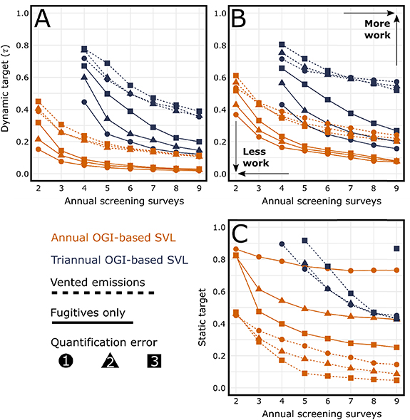
Figure 2. Catalogue of equivalence scenarios under various conditions: (A) dynamic targets assuming leak-rate distribution D1 (more skewed), (B) dynamic targets assuming leak-rate distribution D2 (less skewed), and (C) static targets assuming D1. Each point represents an equivalence scenario with either annual (orange) or triannual (blue) OGI-based SVL programs. In general, more screening (either surveys or follow-up) is required to achieve equivalence with SVL programs that have higher survey frequencies. Solid lines assume that all emissions are fugitives, while dashed lines assume the additional presence of vented emissions. Quantification errors increase from  (perfect facility-scale quantification) to
  (order or magnitude error) and are explained in the main text. Note the different interpretations of dynamic targets (
 ; proportion of top-emitting facilities requiring follow-up) and static targets (proportion of the fugitive leak-size distribution to target).
Download figure:
Standard image High-resolution imageTriaging is also impacted by quantification error. With no screening quantification error ( ), facilities can be correctly ranked according to emission rate before follow-up inspectors are dispatched. As quantification error increases to
  and
and  , facilities are ranked not according to their true emissions rate (
 ), but according to the estimated rate (
 ), effectively 'shuffling' the ranking. Whereas the impact of vented emissions is relatively consistent for different survey frequencies, quantification error is more problematic for MVL programs with lower screening survey frequencies. This occurs because quantification errors are a percentage of the true emission rate, whereas vented emissions are drawn from an empirical distribution and are assumed independent of the fugitive emissions at a facility. When screening survey frequency is high, less time passes between surveys, which allows less time for leaks to accumulate. When
  is close to zero, high quantification errors have less absolute impact on
  . Future work should investigate if
  should be estimated as a percentage of
  or as an absolute difference.
Comparing panels A and B in figure 2 illustrates the impact of leak-size distribution. Equivalence scenarios are achieved with less work for screening programs under D1, which is more heavily skewed (figure 2(A)). When a smaller number of large leaks comprise the majority of total emissions, strategies that focus on these leaks benefit. Figure 2(B) shows equivalence scenarios under the D2 leak-rate distribution, which is less heavy-tailed and consequently requires a larger number of follow-up inspections to achieve equivalence.
Figure 2(C) shows equivalence scenarios using static targets, and must be interpreted differently from panels A and B. Both vented emissions and quantification error result in lower required targets. When vented emissions are added to fugitive emissions at a facility, it makes it easier for the static threshold to be surpassed. However, this results in much more work, which is not immediately evident as a higher static target does not correspond intuitively with follow-up requirements like it does with a dynamic target. Lower static targets are required to achieve equivalence as quantification error increases due to the heavy-tailed shape of the facility-scale emissions distribution. More facilities will fall below a given follow-up threshold than above, meaning that quantification error will push lower-emitting facilities above the threshold more often than higher-emitting facilities below the threshold. This results in more work being done than necessary, leading to a lower static target.
Previous studies have shown the influence of LPR on simulation results (Kemp et al 2016, Fox et al 2021). We present simulations under a range of LPRs to determine whether results in this study are sensitive to LPR (figure S1). Fugitive emissions vary greatly between programs, but because emissions increase for both the SVL and MVL programs, equivalence scenarios are robust to differences in LPR.
3.2. Cost-effectiveness
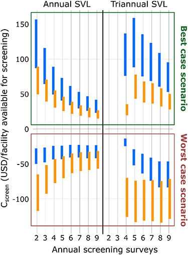
In figure 3, we estimate  for
for  = 0 (blue) and 0.3 (orange) where
  = USD 250/facility (lower limit) and USD 450/facility (upper limit). Under best-case scenarios for MVL, which assume no vented emissions,
  , and D1 (extreme skew),
  rarely exceeds USD 100/facility. To reduce costs relative to the SVL program by 30%, screening costs must not exceed USD ∼50–90/facility. The worst-case scenario is more realistic; it accounts for vented emissions, quantification error (
 ), and assumes D2, which better approximates emissions elsewhere (Brandt et al
2016). Every screening program under the worst-case scenario is more expensive (i.e. negative values) than SVL before screening is paid for. In other words, triaging is so inefficient that, to achieve equivalence, more follow-up surveys must be conducted than would be required under the exhaustive but less frequent SVL program. To illustrate how
), and assumes D2, which better approximates emissions elsewhere (Brandt et al
2016). Every screening program under the worst-case scenario is more expensive (i.e. negative values) than SVL before screening is paid for. In other words, triaging is so inefficient that, to achieve equivalence, more follow-up surveys must be conducted than would be required under the exhaustive but less frequent SVL program. To illustrate how  can be negative, consider a hypothetical LDAR program with 100 facilities. An SVL program that requires annual OGI will require 100 inspections. A proposed MVL program with biannual surveys will have
  if 50 follow-up surveys are required after each survey (
 ), as the total number of follow-up surveys (100) equals the number of required surveys under the SVL program. Therefore,
  for the biannual screening program can only be positive when
  . If screening quantification error reduces triaging effectiveness by introducing triaging errors,
  may increase above 0.5, causing
  to drop below zero.
Figure 3. Maximum screening program costs ( ) under a range of equivalence scenarios. High
  values indicate more cost-effective MVL programs. Estimates are made assuming OGI survey costs of USD $250/facility (lower limit of each line) and USD $450/facility (upper limit of each line). Blue lines show required screening costs when screening program target costs are equal to those of the SVL program (
 = 0). Orange lines show required screening costs for screening programs that offer a 30% cost reduction relative to the SVL program (
 = 0.3). The best-case scenario for MVL assumes perfect screening quantification (
 ), leak rates from D1, and no vented emissions. The worst-case scenario assumes
  , D2, and presence of vented emissions. Negative
  values indicate that screening technology providers must pay to perform services, a situation unlikely to exist in practice.
Download figure:
Standard image High-resolution image
In general, the screening programs simulated in this study are more cost-effective when: (a)  is higher; (b) equivalence scenarios with fewer screening surveys are used (i.e. those with higher
  and more follow-up); (c) vented emissions are lower; (d) quantification error is low; and (e) leak-size distributions are more skewed. Results also suggest that more money is available for screening when SVL program requires more OGI surveys. This is likely due to the relative burden of going from one to two surveys being greater than the burden of going from three to four.
Our results suggest that MVL methods may struggle to be cost-effective compared to conventional OGI-based SVL (figure 3). Vented emissions and quantification errors can lead to incorrect ranking of facilities by emission rate, which increases the required number of follow-up inspections to achieve equivalence. Simulations suggest that MVL will be more cost-effective if triaging errors can be reduced. While negative  values are clearly unprofitable (screening providers would have to pay to provide their service), it is difficult to infer profitability when screening must be USD 50–100 per site. Screening technologies are variable in approach as the industry is nascent and is repurposing technologies used outside the O&G industry. For example, satellites are expensive to build, launch, and operate, but are not constrained by access to services such as lodging for crews and road access. Vehicle-based systems are constrained by driving time but are more scalable as hardware and deployment are less expensive than satellites. These two examples are ends of a spectrum; many variables affect the cost of screening surveys, which may be unprofitable in some contexts while profitable in others.
The scenario with parameters least favourable for MVL viability ('worst-case scenario') considered in this study may overly optimistic due to five modeling assumptions. First, our analysis does not consider the presence of false positive and false negative detections for screening technologies, which could introduce additional triaging errors. False positive and false negative detections exist among screening methods but are more common when the emission rate is close to zero (Ravikumar et al
2019). False negatives are less likely to occur with the largest and most consequential emission sources as detection probability increases with emissions rate (Ravikumar et al
2019). Second, new work is increasingly pointing to temporal variability of methane emissions as a major challenge for mobile LDAR methods that acquire only a 'snapshot' of emissions (Alden et al
2020, Cardoso-Saldaña et al
2020). Here, simulations account for temporal variability of vented emissions, but not of fugitive emissions. If fugitive emissions are episodic, then problems arise for MVL including (a) detecting an episodic fugitive and dispatching a follow-up inspector who is unable to identify the source, and (b) failing to detect an episodic source that was not emitting at the time of screening. For MVL to be effective, the facilities that receive follow-up must be the highest-emitting facilities over time and must be clearly distinguishable from low-emission facilities. Given that screening is a snapshot in time, the implicit assumption is that instantaneous emissions are representative of the long-term average, which may not be the case (Johnson et al
2019). Third, follow-up OGI could be more expensive than OGI used in SVL because flagged facilities may be spaced further apart, which increases travel time and cost. Fourth, this study assumes that screening surveys are spaced evenly apart throughout the year and that they are not impacted by adverse environmental conditions, seasonal variability, or logistical constraints. However, all screening methods have specific operational limitations that may further impact performance, such as clouds for satellites, roads for vehicle systems, snow for LiDAR, and wind and precipitation for drones (Fox et al
2019a). Fifth, we assume that screening technologies have minimum detection limits sufficient to accurately rank at least as many facilities as require follow-up. However, the most cost-effective scenarios require a small number of screening surveys with considerable follow-up ( up to 0.8 for triannual SVL equivalence). When
  is higher, the corresponding minimum detection limit required by the screening method is lower.
Despite these challenges, there may be opportunities for screening technologies. First, our results apply when fugitive emissions are the only target of reductions. New regulations and voluntary reduction initiatives by industry may use screening technologies not specifically for LDAR, but to understand total facility-scale emissions. If so, vented emissions will go from being 'noise' to part of the 'signal' and will not complicate triaging. Second, vented emissions may decline significantly over the coming decades as regulators and industry work towards mitigation targets. Clear steps can be taken to reduce vented emissions, such as conversion from high- to low-bleed pneumatics, installation of vapour recovery units on storage vessels, and best practices for well completions and manual liquid unloadings. These efforts should increase the relative strength of the fugitive signal, assuming no change in leak production rates and LDAR, but may require more sensitive technologies to detect smaller emissions. Third, screening technologies in this study measure only at the facility scale. In reality, many screening technologies may measure at the equipment scale, and the additional granularity could possibly improve MVL. Fourth, we do not consider the cost of repair, as it is assumed that all leaks are eventually repaired, whether the result of an LDAR program or by an operator. However, SVL may lead to higher repair costs, especially as a larger number of smaller leaks are targeted. Fifth, our results are sensitive to the skewness of leak-size distributions, with heavier tails favouring MVL. Production regions, facility types, or other contexts that exhibit extreme heavy tails may therefore benefit the most from MVL.
It may also be possible to reduce triaging errors with better ranking algorithms. The simple static and dynamic thresholds used here are intuitive yet crude; more complex models may be developed that incorporate facility-specific quantification errors and knowledge. For example, if estimated emissions exceed production, it may be possible to identify an error and require additional measurements. However, complex follow-up schemes that are not codified can be difficult to regulate. It is important to note that these results are interpreted in the context of LDAR. Another option is attempting to predict vented emissions from equipment inventories and operator logs to calibrate high-venting sites and improve ranking. MVL technologies may also provide additional value beyond the immediate goal of mitigating fugitive emissions. For example, facility-scale emissions data, even if inaccurate, may be desirable for producers for reporting, tracking progress, or estimating probability of non-compliance with facility-scale venting limits. Some screening technologies can also produce ancillary data for facilities, such as mapping products from vehicles, drones, and aircraft. Screening can also be performed passively if measurement systems are deployed on existing vehicles.
Reducing quantification error for screening technologies may also improve MVL but is a major challenge. Atmospheric variability is a significant source of error (Caulton et al
2018). Accurate wind measurement is also critical in emissions modeling. Some mobile methods have reduced quantification error by increasing measurement times (Brantley et al
2014) or by installing wind sensors on site. However, increased measurement times or requiring wind measurements at every site come with a cost penalty. Additional work will be required to understand whether the trade-off between these factors and quantification error can be sufficiently reconciled to enable cost-effective screening. Possible workarounds may exist. For example, low-sensitivity screening methods may opt for  , eliminating the need for triaging and thus avoiding incorrect ranking. However, minimum detection limits must be consistent for screening methods to ensure that all facilities emitting above a specified amount receive follow-up. It should be noted that this study did not consider systematic bias in quantification errors, which have been observed in previous studies (e.g. Ravikumar et al
2019). While systematic bias should not impact the relative ranking of facility emission rates, this topic warrants further study.
, eliminating the need for triaging and thus avoiding incorrect ranking. However, minimum detection limits must be consistent for screening methods to ensure that all facilities emitting above a specified amount receive follow-up. It should be noted that this study did not consider systematic bias in quantification errors, which have been observed in previous studies (e.g. Ravikumar et al
2019). While systematic bias should not impact the relative ranking of facility emission rates, this topic warrants further study.
More research is required to understand the ways in which mobile screening technologies might contribute to methane monitoring and mitigation. Considerable testing is underway to better understand how a broad variety of different technologies might contribute to reducing methane emissions (Bell et al 2020, Zimmerle et al 2020). Better MVL performance can result from stricter venting limits, improved sensors and quantification algorithms, and a better understanding of how, where, and when to use MVL. Close-range systems may also continue to evolve to have better performance than those considered in this study. It should be noted that this study only applies to facility-scale MVL, and that additional analyses are needed to evaluate equipment-scale screening, continuous monitoring, single-visit screening models, and other approaches to alternative LDAR.
4. Conclusion
This study used LDAR-Sim—an agent based numerical LDAR model—to explore scenarios involving screening technologies. Our results suggest that (a) emissions-reduction equivalence is possible between SVL and MVL programs, and (b) cost-effective equivalence scenarios exist but may be difficult to achieve. Circumstances that impact performance also impact cost-effectiveness, as more surveys are required to achieve equivalence. We have shown that these circumstances include vented emissions, quantification error, and the empirical leak-size distribution used for modeling.
Our simulations suggest the largest impediment to cost-effective MVL is the confounding presence of vented emissions. Placing tight regulatory focus on leaks only, instead of all methane emissions from a facility, may limit uptake of screening. The primary issue is scale—to find leaks on a facility with extensive vented emissions requires fine-scale measurements, which favours SVL. In terms of chemistry and environmental impact, vented and fugitive methane at any one facility are usually identical. Facility-scale screening technologies could be more effective if the fugitive-vented emissions dichotomy was replaced with a more general focus on identifying and resolving the highest-emitting facilities. However, this shift may hinge on improvements in the quantification accuracy of screening technologies.
Acknowledgments
We acknowledge Alberta Innovates for a Technology Futures scholarship to TAF and NSERC for a Vanier scholarship to TAF.
Data availability statement
Supplementary information contains: (a) all model code, data inputs, and outputs; (b) a comprehensive reproducibility guide to enable transparent reproduction of study results; (c) a sensitivity analysis for leak production rate.
The data that support the findings of this study are openly available at the following URL/DOI: https://github.com/tarcadius/Fox_etal_2021_ERL.