

Abstract
East Africa is a key location for wetland emissions of methane (CH4), driven by variations in rainfall that are in turn influenced by sea-surface temperature gradients over the Indian Ocean. Using satellite observations of CH4 and an atmospheric chemistry-transport model, we quantified East African CH4 emissions during 2018 and 2019 when there was 3-σ anomalous rainfall during the long rains (March–May) in 2018 and the short rains (October–December) in 2019. These rainfall anomalies resulted in CH4 emissions of 6.2 ± 0.3 Tg CH4 and 8.6 ± 0.3 Tg CH4, in each three month period, respectively, and represent a 10% and 37% increase compared to the equivalent season in the opposite year, when rainfall was close to the long-term seasonal mean. We find the additional short rains emissions were equivalent to over a quarter of the growth in global emissions in 2019, highlighting the disproportionate role of East Africa in the global CH4 budget.
Export citation and abstract BibTeX RIS

Original content from this work may be used under the terms of the Creative Commons Attribution 4.0 license. Any further distribution of this work must maintain attribution to the author(s) and the title of the work, journal citation and DOI.
1. Introduction
The atmospheric concentration of methane (CH4), an important greenhouse gas, has continued to rise through the 20th century with only a brief respite early this century between 2000 and 2007. In recent years, there has been particularly strong global mean annual growth, partly driven by pan-tropical variations due to the 2014/2015 El Niño (Zhang et al 2018). Generally, these observed variations have defied any definitive explanation with several competing plausible hypotheses that attribute most changes to a particular emission source (e.g. fires, wetlands, oil and gas, agriculture), or to changes in the oxidation loss by the hydroxyl radical (Rigby et al 2017, Worden et al 2017, McNorton et al 2018, Turner et al 2019, Saunois et al 2020). In practice, on a global scale some combination of changing emissions and loss terms are likely responsible. Previous studies have used a range of data to examine changes on large spatial scales, and the newer satellite data, in particular, provide constraints on regional emission estimates (Hu et al 2018, Lunt et al 2019).
Recent work has highlighted the important role of East Africa in the global CH4 budget (Lunt et al 2019). The primary sources of CH4 in Africa are largely microbial with wetlands, agriculture and waste sources contributing an estimated 65% of total emissions (Saunois et al 2016). Wetlands emit CH4 due to the decomposition of organic matter under anaerobic conditions. At large scales, wetland emissions can be broadly explained by three main controls: temperature, carbon availability and water table depth (Moore et al 1998, Christensen et al 2003, Gedney 2004, Bloom et al 2010). In the tropics, where temperature is less of a limiting factor, the dominant control is water table depth (Bloom et al 2010, Bloom et al 2012, Lunt et al 2019). Precipitation anomalies that help drive changes in the water table are linked to wetland CH4 emission anomalies (Pandey et al 2017), taking into account upstream catchment areas and other basin hydrological factors. Emissions from agriculture, particularly ruminants, may also be affected by water controls. Previous work has shown a strong relationship between dry matter intake and CH4 production in forage-fed cattle (Charmley et al 2016). In East Africa, seasonal changes in the availability of feed affects the seasonal variation of cattle live weight and associated CH4 production (Ndung'u et al 2019).
The wet seasons in East Africa follow the movement of the inter-tropical convergence zone. Northern regions such as Sudan and northern Ethiopia have one wet season which normally peaks in July–September. In contrast regions in the south such as southern Tanzania have a wet season peak in January–March. The region in between, including Kenya and southern Ethiopia, experiences two main wet seasons in March–May (MAM) and October–December (OND) (Herrmann and Mohr 2011). These two wet seasons are termed the long rains and short rains, respectively, and are the focus of this paper.
Large changes in the atmospheric growth of CH4 in 2019 (Dlugokencky 2020) coincided with an extreme positive index of the Indian Ocean Dipole (IOD) (Lu and Ren 2020). A positive IOD index corresponds to warmer ocean temperatures in the western Indian ocean and cooler temperatures in the eastern Indian Ocean (Saji et al 1999). In 2019 this resulted in monthly East African precipitation levels during OND that were one of the wettest short rains seasons on record (Wainwright et al 2020). This followed anomalously high precipitation levels during the MAM 2018 long rains (Kilavi et al 2018). Here, we use satellite observations of CH4 from two independent instruments to investigate the impact of these precipitation anomalies on CH4 emissions from East Africa.
2. Data and methodology
2.1. Satellite data
Two CH4 satellite datasets are used in this study to examine changes over East Africa: TROPOMI and GOSAT. TROPOMI measures, amongst others, short wave infrared (SWIR) radiances around 2.3 µm. To calculate column-averaged CH4 concentrations (XCH4) a physics-based retrieval is used, making use of the Oxygen A-band around 760 nm to infer information about the scattering properties of the atmosphere. The satellite is in a Sun-synchronous orbit with an overpass time of 13:30 local solar time. TROPOMI has a swath width of 2600 km and a ground pixel of 7 × 7 km2. We use the scientific CH4 data product (Lorente et al 2020), which implements the RemoTec retrieval algorithm (Butz et al 2011, Hu et al 2016), and use bias-corrected XCH4 in our analysis, with the bias correction supplied in the data (Lorente et al 2020). Only data with a quality flag of greater than 0.5 are used, which filters data for clouds, high solar and viewing zenith angles and high aerosol loading. In addition we filter the data based on where the SWIR surface albedo is in the range 0.05–0.30, the aerosol optical thickness (AOT) is less than 0.1, and the standard deviation of surface topography in each retrieved pixel is less than 60 m. Initial tests revealed some anomalously low value data values surviving through these filters, so we further filter the data based on where the difference between observed values and the simulated model background levels within the domain are greater than −5 ppb. We use data over the spatial domain of our model simulations which covers −36 to +20∘ N and −20 to 55∘ E.
GOSAT is in a Sun-synchronous orbit with a local equator crossing time of 13:00, resulting in global coverage every three days (Kuze et al
2009). We use data from the Thermal And Near infrared Sensor for carbon Observations—Fourier Transform Spectrometer (TANSO-FTS) that measures short wave infrared (SWIR) radiances between 0.76 and 2.0 µm at a resolution of 0.3 cm−1 (Parker et al
2011). We use the University of Leicester's (UoL) v9 GOSAT-OCPR proxy XCH4 product (Parker et al
2020a). This retrieval algorithm uses a different approach to TROPOMI to calculate XCH4, relying on the co-retrieved CO2 column. Taking the ratio between CH4 and CO2 can account for factors that impact the retrievals, such as aerosol and cloud scattering. An advantage of this proxy approach is that it is more robust than the full physics approach in the presence of clouds and aerosols. However, the proxy approach does rely on having good knowledge of the true CO2 distribution in the atmosphere, and errors in this could impact on the derived XCH4 values. As such, both the full physics and proxy approaches have their strengths and weaknesses. Due to the greater spatial coverage of TROPOMI the number of successful retrievals is far greater than from GOSAT (figure S1). Both datasets have been validated against ground-based data from the Total Carbon Column Observing Network (TCCON) (Wunch et al
2011). For both datasets we average the data into  pixels to create a set of super-observations at a resolution consistent with the GEOS-Chem atmospheric transport model.
Rainfall data in this study are taken from the TAMSAT (v3.1) monthly precipitation dataset (Maidment et al 2014, Tarnavsky et al 2014, Maidment et al 2017). The data are based on high-resolution thermal-infrared observations and available from 1983 to the present. Rainfall anomalies reported in this work are relative to the 1983–2012 monthly mean. To examine changes in terrestrial water storage we use data from the GRACE Follow-On (GRACE-FO) mission (Landerer et al 2020). The GRACE-FO dataset provides monthly liquid water equivalent (LWE) estimates at a resolution of 3∘ × 3∘. Anomalies are relative to the consistent longer-term GRACE dataset 2002–2017 monthly means.
2.2. GEOS-Chem chemistry transport model
We use the GEOS-Chem chemistry transport model to simulate the emissions and transport of atmospheric methane (Bey et al
2001, Turner et al
2015). The model was run in a nested configuration with a spatial resolution of 0.25 driven by offline meteorology fields from the GEOS-FP analysis product. The model has 47 vertical levels. The temporal resolution of the meteorology fields was hourly and the transport and chemistry time steps were five and ten minutes respectively. The nested domain covered −36 to 20∘ N and −20 to 55∘ E, encompassing sub-Saharan Africa.
A priori CH4 emissions within the nested domain mostly followed those used in previous published work (Maasakkers et al 2019), with anthropogenic emissions for 2012 from EDGAR v4.3.2, and wetland emissions for 2015 from the WetCHARTs dataset (Bloom et al 2017). Wetland emissions varied monthly and the anthropogenic emissions included a monthly varying seasonal cycle for manure emissions and rice. Daily biomass burning emissions for 2018–2019 were taken from the GFAS database (Kaiser et al 2012). Offline loss fields were included accounting for oxidation by the hydroxyl and chlorine radicals, as well as soil absorption (Wecht et al 2014).
Boundary conditions to the nested domain were created from a global run of the GEOS-Chem model run at 2∘ × 2.5∘, with 3 h output fields. These fields were sampled at the time and location of GOSAT data, and column average XCH4 values compared to the data after applying the GOSAT averaging kernels. To create more realistic boundary condition fields that were consistent with the observed zonal distribution of CH4, these model fields were then scaled to match the GOSAT zonal monthly mean concentrations within a domain of −50∘ E to 100∘ E, encompassing data over the Atlantic and Indian oceans. GOSAT data from within the nested African domain were not included in this zonal mean comparison to avoid using these data twice.
The zonal mean of each 2∘ latitudinal grid cell in the model is thus consistent with the equivalent zonal mean of GOSAT data. However, the vertical and longitudinal distributions of the field are reliant on the a priori emissions fields and GEOS-Chem model transport. The boundary conditions thus represent a reasonable approximation to the true atmospheric field at the boundaries of the nested domain and are consistent with the satellite data which is important to negate any global or latitudinal biases in the data or model. The same boundary conditions were used for both TROPOMI and GOSAT inversions, although due to an offset between the two satellites the boundary conditions from TROPOMI were adjusted according to the global mean ratio between the two satellite datasets each month. The impact of using alternative boundary condition fields on our results is explored in the supplementary material (available online at stacks.iop.org/ERL/16/024021/mmedia).
2.3. Emissions estimation
To estimate CH4 emissions we use an Ensemble Kalman Filter (EnKF) system. Here, we use a variant called the Local Ensemble Transform Kalman Filter (LETKF) (Hunt et al 2007) which has been applied in various previous atmospheric inversions to infer emissions (Miyazaki et al 2012, Liu et al 2016). We briefly describe the LETKF here, and refer the reader to Hunt et al (2007) for an in-depth description.
The LETKF transforms a background ensemble of emissions  with k ensemble members into an analysis ensemble
  . The emissions ensemble is defined by its mean
  and ensemble perturbations
  given by:

The GEOS-Chem model is used to create the operator, H that propagates the emissions ensemble into the observation space following:

Ensemble perturbations in the measurement space,  , are similarly defined to the emissions space as:

The background ensemble,  , is updated to an analysis ensemble
  , based on the data,
  , and calculated by:

where  is the observation error covariance matrix, and
  its matrix inverse.
  is the local analysis error covariance matrix estimated in the ensemble space, and given by:

The updated ensemble perturbations can be calculated according to:
Finally, the a posteriori analysis error covariance matrix is equal to:
The diagonals of  represent the uncertainties of the a posteriori emissions. In our implementation of the LETKF, the state vector,
  , describes a vector of scale factors applied to the a priori emissions field, with each term in
  representing a box of horizontal dimension
  . Our a posteriori emissions are calculated by multiplying the a posteriori scale factors by the a priori emission magnitudes. Unless otherwise stated, all results represent total CH4 emissions from the sum of all sources.
We used an ensemble of 140 members, a temporal assimilation window of 15 days, and lag window of 1 month. A priori emission uncertainties of each grid cell were set to be 200% of the value of each grid cell. In the LETKF, we applied a spatial localization of 800 km that limits the set of observations that are used in the analysis of each state vector element to be within this distance. The diagonal terms of the measurement covariance matrix,  , were formed from a combination of the measurement retrieval a posteriori uncertainties provided in the TROPOMI and GOSAT data files and a modelling uncertainty of 4 ppb, based on the global mean bias of the satellite columns versus TCCON data (Lorente et al
2020, Parker et al
2020a). We defined off-diagonal terms of
, were formed from a combination of the measurement retrieval a posteriori uncertainties provided in the TROPOMI and GOSAT data files and a modelling uncertainty of 4 ppb, based on the global mean bias of the satellite columns versus TCCON data (Lorente et al
2020, Parker et al
2020a). We defined off-diagonal terms of  , to follow an exponential spatial covariance that decayed with a length scale of 50 km. We tested the impact of the inversion parameter definitions on our results through a series of sensitivity tests (see supplementary material).
3. Results
3.1. Rainfall anomalies over East Africa
Between December 2017 and December 2019 there were two notable positive rainfall anomalies: the long rains season of MAM 2018, and the short rains season of OND 2019 (figure 1(a)). The long rains anomaly in 2018, peaked in April with 86 mm month−1, relative to the 1983–2012 mean. The short rains anomaly in 2019, peaked in October with 81 mm month−1. The standard deviation of monthly anomalies over the 38-year self-consistent data record was 17 mm month−1 so that both rainfall anomalies exceed the 3σ level, approximately equivalent to a once in a 30-year event. The 30-year mean rainfall peak in April was 88 mm month−1, and 67 mm month−1 in October, showing that these anomalies represent at least double the normal amount of rainfall across the region.
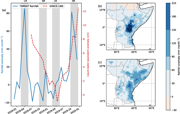
Figure 1. (a) Monthly mean rainfall anomalies from TAMSAT averaged across East Africa (blue) and GRACE liquid water equivalent height anomalies (red). The grey vertical bars indicate the 4 wet seasons during the period 2018–2019. The lines represent the mean of the filled contour region in the two right panels. LR = long rains; SR = short rains. (b) The spatial distribution of mean rainfall anomalies in MAM 2018. (c) The spatial distribution of mean rainfall anomalies in OND 2019.
Download figure:
Standard image High-resolution imageThese two large seasonal anomalies had contrasting spatial distributions. The MAM 2018 anomalies were principally over Kenya, Tanzania and Ethiopia (figure 1(b)), while the anomalies during OND 2019 were also over Somalia, Uganda and South Sudan (figure 1(c)). In contrast the wet seasons in OND 2018 and MAM 2019 were close to climatological mean values, with mean anomalies of −3 mm month−1 in both OND 2018 and MAM 2019.
A similar, albeit smoother, pattern of anomalies is seen in liquid water equivalent (LWE) height anomalies in East Africa from the GRACE-FO mission (Landerer et al 2020) (figure 1(a)), between 2018–07 and 2019–12. The data show a minimum reached in 2019–04, before an increase in the latter part of 2019. Previous studies used LWE anomalies to isolate wetland emissions of CH4 using satellite column measurements of CH4 (Bloom et al 2010, Bloom et al 2012), implying likely changes in wetland emission anomalies as a result of the LWE changes during this period.
3.2. XCH4 enhancements from TROPOMI
Corresponding seasonal mean XCH4 enhancements over East Africa (figure 2) are calculated by subtracting a model background component from the XCH4 column. The model background component is generated by including only that part of the modelled CH4 field that originated from outside the regional domain in the GEOS-Chem simulation. We assume that the dominant factor affecting XCH4 enhancements is surface emissions, acknowledging that any errors in generating the modelled background component will affect this quantity. Gaps in the XCH4 data are due to cloud coverage, surface albedo or aerosol interference preventing successful retrievals; some seasonal mean values may be indicative of only a few successful retrievals in that season (figure S2).

Figure 2. Mean TROPOMI XCH4 enhancements averaged over the 3 months of each wet season in  bins for (a) MAM 2018, (b) MAM 2019, (c) OND 2018, (d) OND 2019. The enhancement is calculated by subtracting the column averaged model background from the observed satellite total column average.
Download figure:
Standard image High-resolution imageWe find the largest XCH4 enhancements over the Sudd wetlands in South Sudan and the Sobat basin to its east, which are present in OND 2018 and 2019. October represents the end of the wet season in South Sudan, but it is usually the time of peak flooding of the Sudd, due to inflow from the region to the south known as the torrents (Sutcliffe and Parks 1999, Lunt et al 2019). In MAM 2018 large XCH4 enhancements (mean 17 ppb; max 93 ppb) are observed in South Sudan and regions south and east of Lake Victoria. In contrast, in MAM 2019 these regions display smaller enhancements (mean 12 ppb; max 52 ppb) consistent with reduced precipitation and emissions. Similarly, while enhancements (mean 17 ppb; max 65 ppb) are seen during OND 2018, consistent with wetland emissions from South Sudan, even larger enhancements (mean 20 ppb; max 86 ppb) are present in OND 2019, particularly over South Sudan (figure 2). The mean XCH4 enhancements in MAM 2018 and OND 2019 across East Africa are 33% and 18% larger than the equivalent season in the opposite year, consistent with the large positive seasonal precipitation anomalies (figure 1).
3.3. East African CH4 emissions
The enhancements in the satellite data provide a useful indication of potential emission anomalies. However, to fully understand the behaviour of the fluxes a more formal Bayesian inversion is required. XCH4 measurements from TROPOMI and GOSAT were assimilated into the LETKF inversion to provide monthly CH4 emission estimates. The a posteriori CH4 emission estimates corresponding to each set of data are generally consistent within their uncertainties (figure 3). Both sets of estimates show prominent emission peaks during MAM 2018 and particularly OND 2019. Our a posteriori emissions estimate from TROPOMI XCH4 data in MAM 2018 is 6.2 ± 0.3 Tg CH4 and in OND 2019 is 8.6 ± 0.3 Tg CH4. These represent a 0.5 ± 0.2 Tg CH4 (10%) and 2.3 ± 0.2 Tg CH4 (37%) increase from MAM 2019 and OND 2018, respectively. We calculate similar a posteriori seasonal emissions inferred from GOSAT XCH4 data of 6.4 ± 0.5 Tg CH4 and 8.1 ± 0.5 Tg CH4 in MAM 2018 and OND 2019, respectively, with an emissions difference in OND of 2.1 ± 0.3 Tg CH4 and a larger MAM difference of 1.2 ± 0.3 Tg CH4 (table S1).
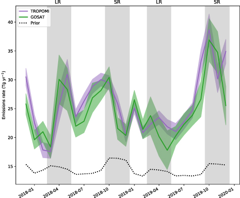
Figure 3. Monthly emissions rate (Tg CH4 yr−1) from East Africa showing a posteriori emissions from inversions using TROPOMI data (purple) and GOSAT inversion results (green). A priori emissions are shown in black. The grey vertical bars indicate the 4 wet seasons during the period 2018–2019. LR = long rains; SR = short rains.
Download figure:
Standard image High-resolution imageThe additional seasonal pulses of CH4 emissions in MAM 2018 and OND 2019 coincide with large growth rates of global atmospheric CH4 of 8.5 ppb and 10.4 ppb in 2018 and 2019 respectively (Dlugokencky 2020). By incorporating these global mean CH4 data into a one box-model calculation, global emissions growth is estimated to be 5 and 7 Tg CH4 in the respective years, assuming a constant atmospheric lifetime (see appendix and figure S3). Therefore, the additional seasonal emissions pulses we report from East Africa, based on TROPOMI (GOSAT) data, represent 10 (24)% and 32 (30)% of the increase in global CH4 emissions in 2018 and 2019 respectively. Although our calculation is subject to assumptions regarding the atmospheric loss rate of CH4 it demonstrates that the seasonal East African emission pulses could account for a considerable fraction of the global emissions growth in 2018 and 2019.
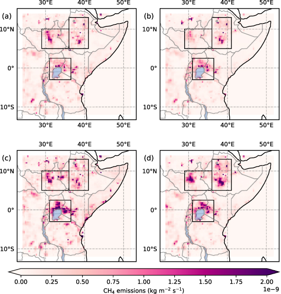
The distribution of OND emissions in 2018 and 2019 from both TROPOMI and GOSAT derived estimates is shown in figure 4. Both estimates show increases in emissions in the region surrounding Lake Victoria. The TROPOMI estimates indicate an increase of 0.7 ± 0.1 Tg CH4 from this region and the GOSAT inversions 0.4 ± 0.3 Tg CH4. The major regions of change from the GOSAT estimates are seen in S Sudan and Ethiopia with two distinct hotspots around 8∘ N. The increase in emissions from the S Sudan regions is 0.4 ± 0.1 Tg CH4, and from Ethiopia 0.8 ± 0.2 Tg CH4. The TROPOMI results indicate a smaller increase of 0.2 ± 0.1 Tg CH4 from both regions, but a change in the emissions distribution, with greater emissions in 2019 around the South Sudan/Ethiopia border in the Sobat basin. Greater emissions from this wetland region to the east of the Sudd, are consistent with significant positive soil moisture anomalies in OND 2019 (figure S4).
Figure 4. Three-month mean a posteriori distribution of CH4 emissions (kg m−2 s−1) from TROPOMI and GOSAT inversions during the short rains (OND) season in 2018 and 2019. (a) TROPOMI 2018, (b) GOSAT 2018, (c) TROPOMI 2019, (d) GOSAT 2019. The boxes indicate the Lake Victoria, S Sudan and Ethiopia emission regions discussed in the text.
Download figure:
Standard image High-resolution image
The simulated background component of the data is consistent between the two observational datasets. Therefore, differences in estimated emissions reflect differences in the spatial coverage and density of observations as well as any offsets in observed XCH4 values. The sparser GOSAT coverage, relative to TROPOMI, can explain why emissions are generally confined to regions where a priori emissions are most prominent (figure S5).
We solve for total CH4 emissions, and cannot directly determine the underlying source sectors behind the seasonal emissions pulses we find. However, we can make the crude assumption that the fractional contribution of each source sector in each grid cell is the same in the a posteriori distribution as in the a priori. Given this assumption, we find that the largest component of the seasonal OND emissions peak in both years is from wetlands emissions (60%) followed by agriculture (15%), based on the difference between a posteriori emissions in OND and June. The division into sector emissions is limited because the a priori source sectors are not spatially distinct (figures S5–S6). However, at a qualitative level it suggests wetlands are the major driver of the a posteriori seasonal OND peak.
To further investigate the impact of the a priori distribution on the estimated short rains emission pulse of 2019 we conducted a sensitivity test, redistributing the wetland component of emissions to follow the soil moisture distribution (figure S7), since errors in the wetland inventory extent have been shown to cause a mismatch to satellite observations (Parker et al 2020b). Using our revised a priori emissions distribution we estimate a posteriori emissions of 8.4 ± 0.4 Tg CH4 in OND 2019 that are close to the estimate (8.6 ± 0.3 Tg CH4) corresponding to the main results, although with a different distribution of emissions (figure S7). We find the East Africa seasonal emission pulses are also relatively insensitive to changes in lateral boundary conditions and various assumptions made in the inversion method (figure S8).
Annual mean total CH4 emission estimates from East Africa for 2018 and 2019 are 25 ± 1 and 27 ± 1 Tg CH4 yr−1 respectively. Our GOSAT derived estimates for both years are 24 ± 1 Tg CH4 yr−1. Results from both satellites are substantially larger than the a priori fluxes, the mean of which is 15 Tg CH4 yr−1 in both years. Through scaling the relative a priori emissions of each source sector in each grid cell by the a posteriori ratio we find that, in June (when emissions are at a minimum) agricultural emissions from livestock account for 60% of this difference between a priori and a posteriori emissions. A sensitivity test using a priori fluxes that are twice as large in all grid boxes returned the same annual mean emissions for East Africa, indicating the minimal impact of a priori emissions on our results at this regional scale (figure S9).
Our East African emissions estimates are slightly smaller than the estimate from previously published work for the 2011–2016 mean of 27 Tg CH4 yr−1 (Lunt et al 2019). We attribute this to differences in emissions from South Sudan. Our annual mean emission estimates for total CH4 from S Sudan are 3.4 ± 0.2 Tg CH4 yr−1 in 2018–2019 from TROPOMI XCH4 data and 3.4 ± 0.3 Tg CH4 yr−1 from GOSAT XCH4 data, compared to the recently published estimates of 6.3 Tg CH4 yr−1 for 2015–2016 (Lunt et al 2019). Assuming a dependency on water table height, these estimates can be reconciled by GRACE LWE height anomalies which dropped from +2.6 cm in 2015–2016 to −1.5 cm in 2018, returning to levels closer to values in 2011–2012 when estimates from this previous study were 3.5 Tg CH4 yr−1 (Lunt et al 2019).
However, our estimates for the sum of all sources from S Sudan are inconsistent with another recent study which estimated emissions from only wetlands of 7.2 ± 3.2 Tg CH4 yr−1 in 2018–2019 using TROPOMI data and a mass balance method (Pandey et al 2020). A bias in the definition of the background concentration used by either approach will lead to larger or smaller XCH4 enhancements and subsequent emission estimates. For instance, our sensitivity tests show that a 5 ppb positive bias in the background results in East African emissions that are larger by 6 Tg CH4 yr−1. However, we find that this bias translates into a S Sudan estimate that is larger by only 0.5 Tg CH4 yr−1, suggesting that the background contribution to the total XCH4 column would have to be substantially smaller to reconcile the two estimates. When we relax our TROPOMI observation selection criteria to closely follow Pandey et al (2020), allowing greater aerosol loading and surface albedo thresholds, our a posteriori estimate for S Sudan increases to 4.6 Tg CH4 yr−1. While this partly helps to reconcile the emission difference the resulting emission distribution is forced to be unrealistic, and inconsistent with results using GOSAT data (supplementary material). A further explanation is likely to lie in the use of different meteorology fields (GEOS-FP vs ERA-5) and the use of a mass-balance method in Pandey et al (2020) versus the 3D modelling and EnKF approach used here.
4. Conclusions
We demonstrate how the extreme rainfall anomalies over East Africa in 2019 in particular, led to additional seasonal emissions of CH4. The positive precipitation anomalies in late 2019 continued into early 2020, resulting in the water levels of Lake Victoria reaching record-breaking levels (Wainwright et al 2020). A previous rapid increase in Lake Victoria water levels in the 1960s was estimated to lead to a doubling of the flooded extent of the Sudd wetlands in South Sudan (Sutcliffe and Parks 1999). Release rates from the dams controlling the outflow of Lake Victoria have been at unprecedentedly high levels in 2020 to mitigate the impacts of lakeside flooding. As a result, due to the greater water flows entering the White Nile we anticipate this should impact CH4 emissions from downstream wetland regions such as the Sudd in the latter half of 2020. In the longer term, with climate models projecting that the frequency of the extreme positive values of the IOD increase under future climate (Cai et al 2018), it is important we take into account the disproportionately large contributions by East Africa to the global growth rate of atmospheric CH4.
Data availability statement
GRACE/GRACE-FO Mascon data are available at http://grace.jpl.nasa.gov. TAMSAT data are available from www.tamsat.org.uk/data. The GOSAT v9.0 dataset is available at https://doi.org/10.5285/18ef8247f52a4cb6a14013f8235cc1eb. The presented material contains modified Copernicus TROPOMI CH4 data, available from ftp://ftp.sron.nl/open-access-data-2/TROPOMI/tropomi/ch4/.
Acknowledgments
MFL and PIP gratefully acknowledge funding from the Methane Observations and Yearly Assessments (MOYA) project (NE/N015916/1) and the National Centre for Earth Observation funded by the National Environment Research Council (NE/R016518/1). The TROPOMI data processing was carried out on the Dutch national e-infrastructure with the support of the SURF Cooperative. RJP and HB are funded via the UK National Centre for Earth Observation (NE/R016518/1 and NE/N018079/1), and acknowledge funding from the ESA GHG-CCI and Copernicus C3S projects. We thank the Japanese Aerospace Exploration Agency, National Institute for Environmental Studies, and the Ministry of Environment for the GOSAT data and their continuous support as part of the Joint Research Agreement. The GOSAT data processing used the ALICE High Performance Computing Facility at the University of Leicester.
Appendix
To estimate the global growth of emissions we used a simple one-box model of the atmosphere. The change in concentration over time through mass balance is given by:
where B is the tropospheric concentration (Tg), Q is the emissions rate (Tg/yr) and k is the loss rate (yr−1), proportional to one over the lifetime. Through integration of equation (A1) and rearrangement it can be shown (Jacob 1999) that the emissions at time, t are equal to:
We used annual mean CH4 mole fraction data from the National Oceanic and Atmospheric Administration (NOAA) (Dlugokencky 2020). We used a conversion of tropospheric mole fraction to mass of 2.767 Tg CH4 ppb−1 (Lassey et al 2007). We tuned the loss rate to match a steady state annual mean concentration of 1775 ppb with emissions in 2002–2006 of 546 Tg CH4 yr−1 (Saunois et al 2017). Based on the NOAA annual mean data and these numbers we estimate global emissions of 586, 591 and 598 Tg CH4 yr−1 in 2017, 2018 and 2019 respectively (figure S3). This represents a 5 and 7 Tg increase in global CH4 emissions in 2018 and 2019 respectively. The box model calculation is highly simplified and assumes a constant loss rate of CH4 from the atmosphere. A decreasing/increasing loss term over time would result in smaller/larger global emission estimates. Even so, at the global scale the mass balance approach provides a reasonable approximation to the evolution of atmospheric CH4, and show the East African emission pulses could account for a considerable fraction of the observed atmospheric growth.