

Abstract
Using state-of-the-art models from the Coupled Model Intercomparison Project Phases 5 and 6 (CMIP5/6), future changes of sudden stratospheric warming (SSW) events under a moderate emission scenario (RCP45/SSP245) and a strong emissions scenario (RCP85/SSP585) are evaluated with respect to the historical simulations. Changes in four characteristics of SSWs are examined in 54 models: the SSW frequency, the seasonal distribution, stratosphere–troposphere coupling, and the persistency of the distorted or displaced polar vortex. The composite results show that none of these four aspects will change robustly. An insignificant (though positive) change in the SSW frequency from historical simulations to RCP45/SSP245 and then to RCP85/SSP585 is consistently projected by CMIP5 and CMIP6 multimodel ensembles in most wintertime months (December–March). This increase in the SSW frequency is most pronounced in mid- (late-) winter in CMIP6 (CMIP5). No shift in the seasonality of SSWs is simulated especially in the CMIP6 future scenarios. Both the reanalysis and CMIP5/6 historical simulations exhibit strong stratosphere–troposphere coupling during SSWs, and the coupling strength is nearly unchanged in the future scenario simulations. The near surface responds immediately after the onset of SSWs in both historical and future scenarios experiments, denoted by the deep downward propagation of zonal-mean easterly anomalies from the stratosphere to the troposphere. On average, the composite circumpolar easterly winds persist for 8 d in the reanalysis and CMIP5/6 historical experiments, which are projected to remain unchanged in both the moderate and strong emissions scenarios, implying the lifecycle of SSWs will not change.
Export citation and abstract BibTeX RIS

Original content from this work may be used under the terms of the Creative Commons Attribution 4.0 license. Any further distribution of this work must maintain attribution to the author(s) and the title of the work, journal citation and DOI.
1. Introduction
Sudden stratospheric warmings (SSWs) are a spectacular phenomenon in the climate system, and are distinguished by warming of the Arctic stratosphere by tens of degrees within a week, reversing the meridional temperature gradient (Charlton and Polvani 2007, Butler et al 2015, Cao et al 2019). During SSWs, variability in the stratosphere is often coupled to that in the troposphere (Karpechko et al 2018, Liu et al 2019, Rao et al 2019). Weakening, displacement, and distortion of the stratospheric polar vortex during SSWs can project onto a negative stratospheric annular mode (Baldwin and Dunkerton 1999, Baldwin et al 2003, Sigmond et al 2013, White et al 2019, 2020, Rao et al 2020). The gradual downward propagation of the northern annular mode (NAM) signal from the stratosphere to the troposphere increases predictability of surface weather on subseasonal timescales (Sigmond et al 2013, Tripathi et al 2015, 2016, Domeisen et al 2020a, 2020b). For example, a cold Eurasian continent–warm North American continent pattern is observed before SSWs in both reanalyses and Coupled Model Intercomparison Project Phase 5 (CMIP5) models, while most parts of those two continents are anomalously cold after SSWs (Thompson et al 2002, Mitchell et al 2013, Lehtonen and Karpechko 2016, Cao et al 2019, Liu et al 2019).
SSWs can be identified by reversal of zonal winds at 10 hPa and 60° N (Charlton and Polvani 2007). Based on the morphology of the stratospheric polar vortex, SSWs are classified into vortex displacement events and vortex split events (Seviour et al 2013, White et al 2019, 2020). Some studies found similar surface impact of displacement and split SSWs (Charlton and Polvani 2007, White et al 2019), while some emphasized their differences (Nakagawa and Yamazaki 2006, Mitchell et al 2013, Seviour et al 2016). Vortex split SSWs show a slightly stronger North Atlantic surface signal in the month following onset (Seviour et al 2013, O'Callaghan et al 2014), while vortex displacements show stronger negative pressure anomalies over Siberia (Seviour et al 2016). Identified difference between impacts of displacement and split SSWs in previous studies might be partially caused by the composite intensity of the SSWs (Rao et al 2020), although the methods, sample sizes, and timescale considered (e.g. daily, weekly, or monthly) also contribute.
Based on these definitions, simulation of SSW events have been widely assessed for CMIP5 (e.g. Charlton-Perez et al 2013, Osprey et al 2013, Seviour et al 2016, Kim et al 2017, Cao et al 2019) and recently for CMIP6 (Liu et al 2019, Ayarzagüena et al 2020) models. It has been reported that high-top models generally exhibit better performance of SSW simulations than the low-top models (Charlton-Perez et al 2013, Osprey et al 2013, Seviour et al 2016, Kim et al 2017), although the threshold of classifying models as either high- or low-top models is somewhat subjective. CMIP5 models can simulate several aspects of SSWs to different degrees of success based on single-model assessment (e.g. HadGEM2 in Osprey et al 2013; CESM1-WACCM in Cao et al 2019) and multimodel studies (e.g. 21 models in Charlton-Perez et al 2013; 13 high-top models in Seviour et al 2016). Low-top models underestimate stratospheric variability on interannual and daily time scales, and both low-top and high-top models cannot produce the decadal variability and a realistic dynamical response to volcanic eruptions in CMIP5 (Charlton-Perez et al 2013). Osprey et al (2013) compared the SSW frequency in two configurations (low-top versus high-top) of HadGEM2, and found that much more SSWs occur in the high-top version of their model than the low-top version (7.2 versus 2.5 per decade).
Due to the possible downward impact of SSWs, their predictability has been the topic of wide interest in literature most recently and their maximum predictive limit is consistently around one to two weeks in those studies (e.g. Karpechko et al 2018, Rao et al 2018, Butler et al 2020, Taguchi 2020, Domeisen et al 2020a, 2020b) though some events may be predictable for longer lead times (Rao et al 2019, 2020).
The possibility of future change in SSWs has attracted wide attention in the past decade though no consensus has been established in literature (Charlton-Perez et al 2008, Mclandress and Shepherd 2009, Bell et al 2010, Karpechko and Manzini 2012, Mitchell et al 2012, Kim et al 2017, Ayarzagüena et al 2018, 2020). Some single-model studies project a significant increase in the frequency of SSWs in the future (e.g. Charlton-Perez et al 2008, Bell et al 2010, Kim et al 2017). On the contrary, some others project no significant change in the SSW frequency (Mclandress and Shepherd 2009, Karpechko and Manzini 2012, Scaife et al 2012). All of these studies compare the change in the SSW frequency in the present-day climate with a warmer future climate due to an increased concentration of greenhouse gases. Based on a multimodel study that minimizes the possible interference of internal variability, Ayarzagüena et al (2018) also found a tiny increase in the future SSW frequency using different SSW identification algorithms in 12 models, but such a change was found to be insignificant. This insignificant change is verified later by the Diagnostic, Evaluation, and Characterization of Klima (DECK) simulations (preindustrial control and quadruple CO2) from the state-of-the-art CMIP6 models (Ayarzagüena et al 2020).
Most CMIP6 models have uploaded their future scenarios simulations, which allows a more natural comparison of CMIP5 and CMIP6. Combining CMIP5 and CMIP6 outputs, we are able to assess the response in 54 models, with the hope of isolating any signal from the noise. We provide more robust evidence to show that although an increase in the frequency of SSWs is projected by multimodel ensemble (MME) both for CMIP5 and CMIP6, such a change is very small and generally insignificant, consistent with some recent reports using around a quarter of the number of models we use here (Ayarzagüena et al 2018, 2020). Note that Ayarzagüena et al (2020) use CMIP6 DECK simulations, we use CMIP5/6 coupled simulations produced by a larger number of models. In addition to the undetectable change in the frequency of SSWs, we consider additional aspect of SSWs that have received less attention. Specifically, we will show that the stratosphere–troposphere coupling during SSWs is little altered in the future projection scenarios, and the change in the seasonal distribution of SSWs is also small.
Organization of the paper is as follows. Following the introduction, CMIP5/6 models, datasets and methods are described in section 2. Several aspects of changes in SSWs are shown in sections 3–5, including the frequency, seasonal distribution, intensity of downward propagation of SSW signals (that is, stratosphere–troposphere coupling) and persistency of easterlies. Finally, results are summarized and discussed in section 6.
2. CMIP5/6 models, datasets and methods
2.1. CMIP5/6 models and experimental datasets
Tables 1 and 2 list CMIP5/6 models used in this study, respectively. To project a change of SSWs in the future, the daily zonal winds are required both for historical and future scenarios simulations for a specific model. At the time of data downloading (January 2020), 37 CMIP5 (table 1) and 38 CMIP6 (table 2) models have daily zonal winds for either/both the historical or/and the two future scenarios simulations. The historical runs refer to the simulation forced by all forcings (i.e. greenhouse gas concentrations, aerosols, ozone depletion, solar cycles, and land uses) in the 20th century (Taylor et al 2012). The historical simulation starts from 1850 and ends in 2005 for CMIP5, whereas it also starts from 1850 but ends in 2014 for CMIP6 due to the time lag between the two projects. The daily outputs for historical simulations are available from 1950 to 2005/2014 for most models, which are used to represent the present-day climate.
Table 1. CMIP5 models used in this study with daily zonal winds available denoted by a check mark (✓). The experiments unavailable are denoted by a cross (×). RCP = Representative Concentration Pathway. Models with all three experiments are marked with an asterisk. Data are publicably available from https://esgf-node.llnl.gov/projects/esgf-llnl.
| Model | Resolution (model top) | Historical | RCP45 | RCP85 |
|---|---|---|---|---|
| ACCESS1.0* | N96L38 (40 km) | ✓ | ✓ | ✓ |
| ACCESS1.3* | N96L38 (40 km) | ✓ | ✓ | ✓ |
| BCC-CSM1-1* | T42L26 (2.917 hPa) | ✓ | ✓ | ✓ |
| BCC-CSM1-1-m* | T106L26 (2.917 hPa) | ✓ | ✓ | ✓ |
| BNU-ESM* | T42L26 (2.917 hPa) | ✓ | ✓ | ✓ |
| CanESM2* | TL63L35 (1 hPa) | ✓ | ✓ | ✓ |
| CCSM4* | F09L26 (2.917 hPa) | ✓ | ✓ | ✓ |
| CESM1-WACCM | F19L66 (5.1 × 10⁻⁶ hPa) | ✓ | × | × |
| CMCC-CESM | F19L39 (0.01 hPa) | ✓ | × | ✓ |
| CMCC-CM* | T159L31 (0.01 hPa) | ✓ | ✓ | ✓ |
| CMCC-CMS* | T63L95 (0.01 hPa) | ✓ | ✓ | ✓ |
| CNRM-CM5* | TL127L31 (10 hPa) | ✓ | ✓ | ✓ |
| CSIRO-Mk3-6-0* | T63L18 (4.5 hPa) | ✓ | ✓ | ✓ |
| EC-EARTH* | TL159L62 (5 hPa) | ✓ | ✓ | ✓ |
| FGOALS-g2* | 128 × 60L26 (2.194 hPa) | ✓ | ✓ | ✓ |
| FGOALS-s2* | R42L26 (2.194 hPa) | ✓ | ✓ | ✓ |
| GEOSCCM | 144 × 90L72 (0.01 hPa) | × | ✓ | × |
| GFDL-CM3 | C48L48 (86.4 km) | ✓ | ✓ | × |
| GFDL-ESM2G* | C48L24 (3 hPa) | ✓ | ✓ | ✓ |
| GFDL-ESM2M* | C48L24 (3 hPa) | ✓ | ✓ | ✓ |
| HadCM3 | N48L19 (10 hPa) | ✓ | ✓ | × |
| HadGEM2-AO | N96L38 (39.2 km) | ✓ | × | × |
| HadGEM2-CC* | N96L60 (85 km) | ✓ | ✓ | ✓ |
| HadGEM2-ES | N96L38 (39.2 km) | × | ✓ | ✓ |
| INMCM4* | 180 × 120L21 (10 hPa) | ✓ | ✓ | ✓ |
| IPSL-CM5A-LR* | 144 × 144L39 (0.04 hPa) | ✓ | ✓ | ✓ |
| IPSL-CM5A-MR* | 96 × 95L39 (0.04 hPa) | ✓ | ✓ | ✓ |
| IPSL-CM5B-LR* | 96 × 95L39 (0.04 hPa) | ✓ | ✓ | ✓ |
| MIROC5* | T85L40 (3 hPa) | ✓ | ✓ | ✓ |
| MIROC-ESM* | T42L80 (0.0036 hPa) | ✓ | ✓ | ✓ |
| MIROC-ESM-CHEM* | T42L80 (0.0036 hPa) | ✓ | ✓ | ✓ |
| MPI-ESM-LR* | T63L47 (0.01 hPa) | ✓ | ✓ | ✓ |
| MPI-ESM-MR* | T63L95 (0.01 hPa) | ✓ | ✓ | ✓ |
| MPI-ESM-P | T63L47 (0.01 hPa) | ✓ | × | × |
| MRI-CGCM3* | TL159L48 (0.01 hPa) | ✓ | ✓ | ✓ |
| MRI-ESM1 | TL159L48 (0.01 hPa) | ✓ | × | ✓ |
| NorESM1-M* | F19L26 (2.917 hPa) | ✓ | ✓ | ✓ |
Table 2. CMIP6 models used in this study with daily zonal winds available denoted by a check mark (✓). The experiments unavailable are denoted by a cross (×). SSP = Shared Socioeconomic Pathways. Models with all three experiments are marked with an asterisk. Data are publicably available from https://esgf-node.llnl.gov/projects/esgf-llnl.
| Model | Resolution (model top) | Historical | SSP245 | SSP585 |
|---|---|---|---|---|
| ACCESS-CM2* | N96L85 (85 km) | ✓ | ✓ | ✓ |
| ACCESS-ESM1-5* | N96L38 (39.2 km) | ✓ | ✓ | ✓ |
| AWI-CM-1-1-MR | T127L95 (80 km) | × | ✓ | ✓ |
| BCC-CSM2-MR* | T106L46 (1.46 hPa) | ✓ | ✓ | ✓ |
| BCC-ESM1 | T42L26 (2.19 hPa) | ✓ | × | × |
| CESM2* | F09L32 (2.25 hPa) | ✓ | ✓ | ✓ |
| CESM2-FV2 | F19L32 (2.25 hPa) | ✓ | × | × |
| CESM2-WACCM* | F09L70 (4.5 × 10⁻⁶ hPa) | ✓ | ✓ | ✓ |
| CESM2-WACCM-FV2 | F09L70 (4.5 × 10⁻⁶ hPa) | ✓ | × | × |
| CNRM-CM6-1-HR* | TL359L91 (78.4 km) | ✓ | ✓ | ✓ |
| CNRM-CM6-1* | TL127L91 (78.4 km) | ✓ | ✓ | ✓ |
| CNRM-ESM2-1* | TL127L91 (78.4 km) | ✓ | ✓ | ✓ |
| CanESM5* | T63L49 (1 hPa) | ✓ | ✓ | ✓ |
| EC-Earth3* | TL255L91 (0.01 hPa) | ✓ | ✓ | ✓ |
| EC-Earth3-Veg* | TL255L91 (0.01 hPa) | ✓ | ✓ | ✓ |
| FGOALS-f3-L | C96L32 (2.16 hPa) | ✓ | × | × |
| FGOALS-g3* | 180 × 80L26 (2.194 hPa) | ✓ | ✓ | ✓ |
| GFDL-CM4* | C96L33 (1 hPa) | ✓ | ✓ | ✓ |
| GFDL-ESM4 | C96L49 (1 hPa) | ✓ | × | ✓ |
| GISS-E2-1-G | 144 × 90L40 (0.1 hPa) | ✓ | × | × |
| HadGEM3-GC31-LL* | N96L85 (85 km) | ✓ | ✓ | ✓ |
| HadGEM3-GC31-MM | N216L85 (85 km) | ✓ | × | × |
| INM-CM4-8* | 180 × 120L21 (10 hPa) | ✓ | ✓ | ✓ |
| INM-CM5-0* | 180 × 120L73 (0.2 hPa) | ✓ | ✓ | ✓ |
| IPSL-CM6A-LR* | N96L79 (80 km) | ✓ | ✓ | ✓ |
| KACE-1-0-G* | N96L85 (85 km) | ✓ | ✓ | ✓ |
| MIROC-ES2L | T42L40 (3 hPa) | ✓ | × | × |
| MIROC6* | T85L81 (0.004 hPa) | ✓ | ✓ | ✓ |
| MPI-ESM-1-2-HAM | T63L47 (0.01 hPa) | ✓ | × | × |
| MPI-ESM1-2-HR* | T127L95 (0.01 hPa) | ✓ | ✓ | ✓ |
| MPI-ESM1-2-LR* | T63L47 (0.01 hPa) | ✓ | ✓ | ✓ |
| MRI-ESM2-0* | TL159L80 (0.01 hPa) | ✓ | ✓ | ✓ |
| NESM3* | T63L47 (1 hPa) | ✓ | ✓ | ✓ |
| NorESM2-LM* | 144 × 96L32 (3 hPa) | ✓ | ✓ | ✓ |
| NorESM2-MM* | 288 × 192L32 (3 hPa) | ✓ | ✓ | ✓ |
| SAM0-UNICON | 288 × 192L30 (2 hPa) | ✓ | × | × |
| TaiESM1 | 288 × 192L30 (2 hPa) | ✓ | × | × |
| UKESM1-0-LL* | N96L85 (85 km) | ✓ | ✓ | ✓ |
The future scenarios are named differently for CMIP5 and CMIP6. It is called Representative Concentration Pathways (RCPs; Taylor et al 2012) with the radiative forcing gradually increasing to a specific representative by 2100 (e.g. 2.6, 4.5, 6, and 8.5 W m−2) for CMIP5. For CMIP6, the future projection is a subproject and named as Shared Socioeconomic Pathways (SSPs; Gidden et al 2019). Considering the availability of model data and the representation of typical forcings, a moderate emission simulation and a strong emission simulation are used in our analysis. Specifically, the climate forcing for the RCP45/SSP245 and RCP85/SSP585 scenarios reach 4.5 and 8.5 W m–2 by 2100, respectively (O'Neill et al 2016). CMIP5 provides RCP45 and RCP85 future scenarios from 2006 to 2100, and CMIP6 provides SSP245 and SSP585 future scenarios from 2015 to 2100. Although the end-date in a few models might exceed 2100 and reach up to 2300, we only use data before 2100 so as to keep the timespan as consistent as possible among models.
We do not exclude low-top models, because (1) low-top models can reproduce SSWs; (2) high-top models also diverge in future projection; and (3) large model size might help to decrease the projection uncertainty. In other words, we do not intend to fully diagnose stratospheric variability in the CMIP5/6 models nor to explain in detail different biases of SSWs in models, both of which have been widely reported in some single-model studies (see the introduction; also see Wu and Reichler 2020). We do however consider the dependence of resolution on SSW frequency in the supplemental material (available online at stacks.iop.org/ERL/16/034024/mmedia).
2.2. Methods
Due to the limitation of our storage and the huge volume of CMIP5/6 data, we mainly focus on the daily zonal-mean zonal winds, which are collected for both CMIP5 and CMIP6. The identification of SSWs uses the WMO definition (Charlton and Polvani 2007), which is based on the reversal of zonal-mean zonal winds at 10 hPa and 60° N. Namely, an SSW is identified if the zonal-mean zonal wind at 10 hPa and 60° N reverse from westerlies to easterlies, and the end of a given SSW must be followed by at least 20 d of westerlies before a subsequent SSW can be identified. Although some minor SSWs might not be identified in some decades using the WMO method for the reanalysis, Palmeiro et al (2015) suggest that the temporal evolution of SSWs is similar using different definitions. The frequency of SSWs is also stable and not so sensitive to the identification algorithm if the data record is long (Butler et al 2015). In addition, using the same criteria for all simulations (historical and future scenarios) might not bias the projected change in SSWs.
Most of our results are based on the MME to decrease the uncertainty of projections based on single-model studies. There are 28 CMIP5 models and 26 CMIP6 models with all simulations (i.e. the historical simulation and two scenarios simulations), and the remaining 9/12 CMIP5/6 models have only one or two of the three simulations. The CMIP5/6 MME is based on the 28/26 models with all simulations (termed 'model group 1'), with the remaining 9/12 CMIP5/6 models without all simulations (termed 'model group 2') excluded from the MME of historical simulations and future scenarios simulations. By focusing on differences between the future scenarios and historical simulation for these 28/26 models included in group 1, we partially are able to cancel out any mean state bias that may exist. The reference state in the present climate system is calculated from a relatively long reanalysis, NCEP/NCAR (1948–2019). We also use the JRA-55 and ERA5 reanalyses and the results are essentially identical (Cao et al 2019). All model data are remapped to the 2.5° × 2.5° (longitude × latitude) global grids to obtain the zonal wind at 60° N, and the results are nearly unchanged if the remapping grid is varied from 1° to 5°.
3. Projected change in the SSW frequency
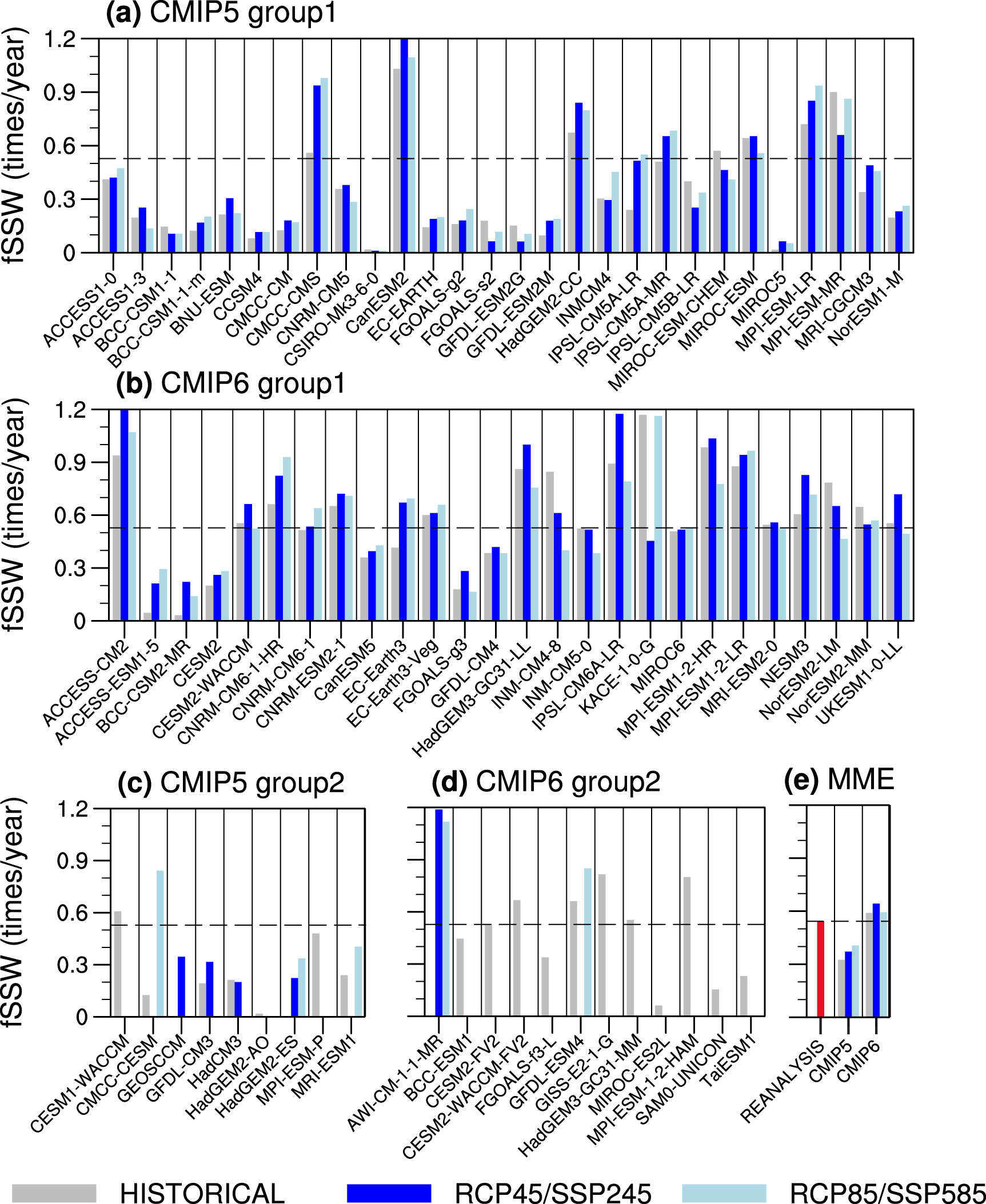
The SSW frequency from CMIP5/6 models is shown in figure 1 for the model group 1 (with full simulations) and model group 2 (lacking one or two simulations), respectively. Most of the CMIP5 models simulate a too-low frequency of SSWs, around 0.3–0.4 events per year in the historical runs (gray bars in figures 1(a) and (c)), with a large inter-model spread from nearly zero in CSIROC-Mk-3-6-0 (also shown in Rao et al (2015) using another SSW definition) and MIROC5 to one SSW per year in CanESM2. Similarly, the SSW frequency simulated in historical runs by CMIP6 also has a large intermodal spread from <0.1 events per year in ACCESS-ESM1-5 and BCC-CSM2-MR to 1.1 events per year in KACE-1-0-G (figures 1(b) and (d)). Comparing CMIP5 and CMIP6, the simulation of SSW frequency is improved based on the MME (figure 1(e)), and specifically the CMIP5 MME shows <0.4 SSWs per year, while CMIP6 MME shows 0.6 SSWs per years more consistent with the reanalysis with 0.5–0.6 SSWs per year on average (Rao et al 2019). Wu and Reichler (2020) document the possible causes for the inter-model variation of the SSW frequency, and they find that the variation in the SSW frequency is related to the strength of the polar vortex and the upward propagating wave activity in the stratosphere. In the supplementary material, it is further revealed that the large inter-model spread of the SSW frequency is related to the intensity of the simulated stratospheric polar vortex, the number of the model vertical levels, and the model top; in contrast, the horizonal resolution shows little impact among CMIP5/6 models on the SSW frequency (figures S1–S8).

Figure 1. Model-by-model frequency of stratospheric sudden warmings (SSWs) from (a), (c) CMIP5 and (b), (d) CMIP6 in the present-day climate system and two future projection scenarios. The present-day climate system is represented by the historical simulation (1850–2005/2014; daily data are typically available from 1950 to 2005/2014; gray bars), with CMIP6 9 year longer than CMIP5 (2006–2014). The two future scenarios (2006/2015–2100) are RCP45/SSP245 (blue bars) and RCP85/SSP585 (light blue bars) from CMIP5/6, with CMIP6 9 year shorter than CMIP5 (2006–2014). Although some models include future projections up until 2200/2300, only model output before 2100 is used here to maintain consistency among the models. Models in group 1 (a), (b) provide all of the three simulations, and those in group 2 do not provide all (only one or two, see the legend). (e) The multimodel ensemble mean (MME) is compared in the last plot with the reanalysis as a baseline (red bar).
Download figure:
Standard image High-resolution imageBoth CMIP5 and CMIP6 models show an inconsistent change of the SSW frequency in the future scenarios. Specifically, some CMIP5 (e.g. BCC-CSM1-1, FGOALS-s2, GFDL-ESM2G, IPSL-CM5B-LR, MIROC-ESM-CHEM, MPI-ESM-MR) and CMIP6 models (e.g. INM-CM4-8, INM-CM5-0, KACE-1-0-G, NorESM2-LR) project a decrease in the frequency of SSWs, while most of remaining models in figures 1(a) and (b) project an increase. Although the MME from CMIP5/6 shows a small increase from the historical simulation to the RCP45/SSP245 scenarios, and then to the RCP85/SSP585 scenarios, such a change is not significant (figure 1(e); t-value < 0.7 for the multi-model mean). The SSW frequency in all of the three simulations from CMIP5 is lower than that from CMIP6, implying a better simulation (and probably a better projection) of SSW frequency in CMIP6. Despite different simulation skills for CMIP5 and CMIP6, the change in sign (+) and magnitude (∼0.05) from the historical simulation to RCP45/SSP245 and RCP85/SSP585 are consistent.
The seasonal distribution of SSWs from November to March is shown in figure 2 for the reanalysis and the three simulations of CMIP5/6. Only the MME is shown for the SSW frequency in each wintertime month. In the reanalysis data, most SSWs happen in midwinter (January–February). As seen from figure 2, there is a common bias for CMIP5 and CMIP6 in simulating SSWs: SSWs tends to occur later than observations, consistent with some previous studies using single-models (e.g. Horan and Reichler 2017, Cao et al 2019, Liu et al 2019), though it is possible that the observed maximum in January is not robust and is rather due to the limited data record (Horan and Reichler 2017). Most SSWs in CMIP5/6 occur in February and March. A similar seasonal distribution is also evident in the future scenario simulations. Therefore, there is little change in the seasonal distribution of SSWs, because both the historical and future simulations show more SSWs in late winter. Finally, we have computed the statistical significance of the future change in SSW frequency for each month separately, and the increase in February and March is statistically significance for the CMIP5 MME even as the increase in the extended winter average is not. However, the increase of the SSW frequency in December and January is statistically significant for the CMIP6 MME. If the low-top models are excluded from the MME, the inconsistent seasonality of the significant change in the SSW frequency between CMIP5 and CMIP6 is still present for high-top models (figure S9). Specifically, the high-top models also project a significant increase in February and March for CMIP5, but the significant increase shifts to December and January for CMIP6 (figures S9(b) and (d)). Hence the month with the biggest increase is not consistent between CMIP5 and CMIP6, and so cannot be considered a robust response even as the increase in a specific month is significant in one of the CMIPs. This issue should certainly be revisited as additional models upload data.
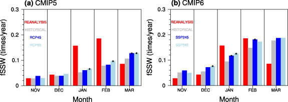
Figure 2. Seasonal distribution of SSWs from November to March in the MME of the historical simulation (gray bars), the RCP45/SSP245 simulation (blue bars), and the RCP85/SSP585 simulation (light blue bars) from (a) CMIP5 and (b) CMIP6. The reanalysis is shown with red bars. The differences between historical simulations and future scenarios projections are significant at the 95% confidence level for a few months, marked with a pentagram over the corresponding scenarios.
Download figure:
Standard image High-resolution image4. Projected changes in stratosphere–troposphere coupling during SSWs
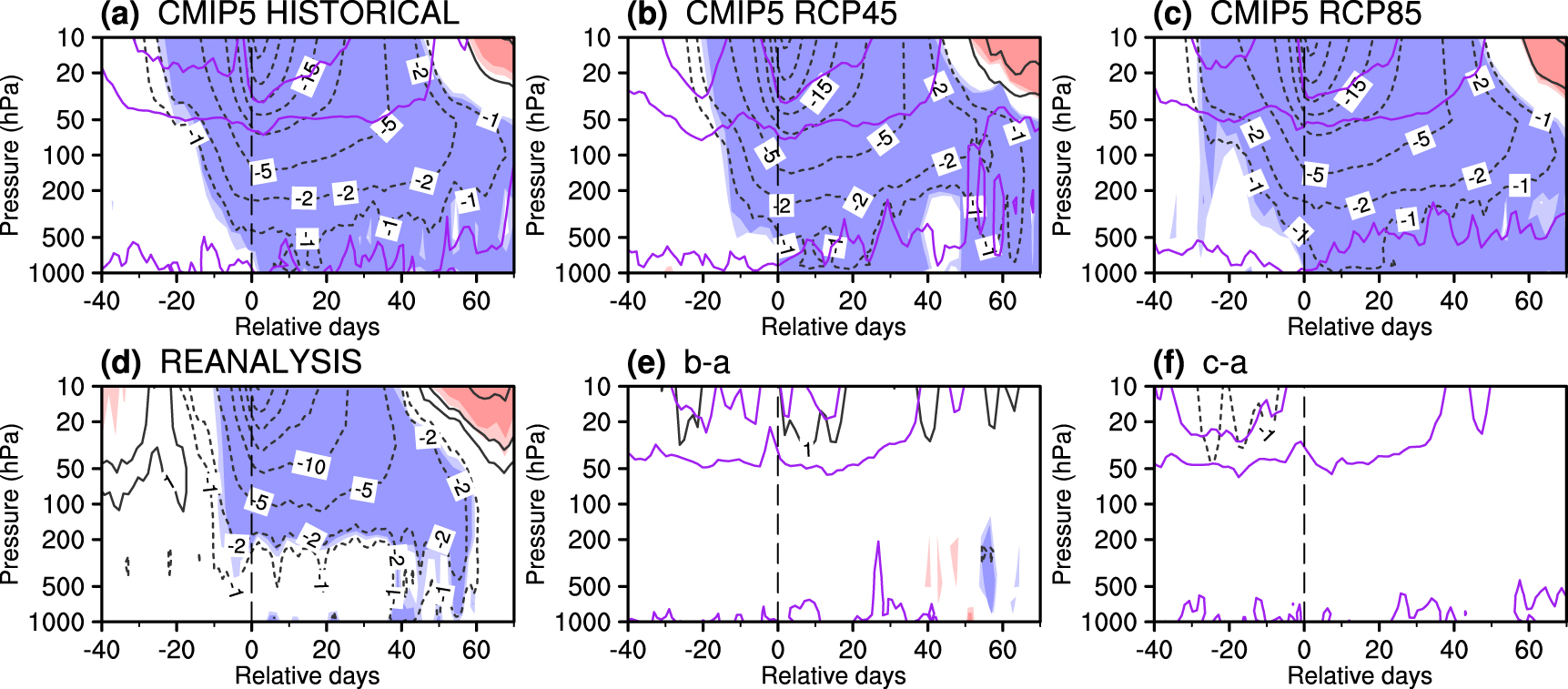
SSWs have been shown to usually lead to the negative phase of the NAM (Baldwin et al 2003, Sigmond et al 2013, Rao et al 2019). Though the NAM is usually represented by either the empirical orthogonal function or the polar cap average of geopotential height, it is closely related to anomalous easterlies in the circumpolar region (e.g. Baldwin and Thompson 2009, Rao et al 2020). To project the future change of the NAM-like response, figure 3 displays the composite pressure–time evolution of the circumpolar easterly anomalies from day −40 to day 70 with respect to the onset date of SSWs for the reanalysis and three scenarios from the CMIP5 MME. With a large sample ensemble, more regions are covered with the 90% and 95% significance levels in models than in the reanalysis (cf figures 3(a) and (d)). Both the reanalysis and CMIP5 historical MME suggest that a deceleration of polar jet has begun on day −20 or earlier, and composite easterly anomalies can persist for more than two months at 10 hPa (day −20 to day 40 or later). The SSW signals show a gradual downward propagation from the stratosphere to the troposphere, and the near-surface response forms after the onset of SSW in both the historical simulation and the reanalysis.

Figure 3. Composite evolutions of SSWs from day −40 to day 70 relative to the onset date of SSWs in (a) the historical simulation, (b) the RCP45 simulation, and (c) the RCP85 simulation. The reanalysis in (d) is shown as a reference for the evolution of SSWs in the present-day climate system. Projected changes of the evolution of SSWs in (e) RCP45 and (f) RCP85 with respect to the historical simulation is shown in the last two plots. Contours are the zonal-mean zonal wind anomalies at 60° N from 1000 to 10 hPa, and light and dark shadings mark anomalies at the 90% and 95% confidence levels, respectively. All plots show the CMIP5 MME. The purple contours show the inter-model standard deviation of the wind anomalies or differences if applicable.
Download figure:
Standard image High-resolution imageThere is no evidence for future changes in the stratosphere–troposphere coupling strength in either scenario from CMIP5 (figures 3(b) and (c)). In the RCP45 MME, the easterly anomalies also begin on day −20 and persist until day 40 at 10 hPa, and the maximum easterly anomalies can reach around −30 m s−1 around day 3 (figure 3(b)). The evolution of the near-surface winds in the RCP45 is also similar to the historical MME, and the near-surface response is simulated shortly after the onset of SSWs. Therefore, no change in the near-surface response to SSWs is projected in RCP45 relative to the historical simulation (figure 3(e)). Similar conclusions are also true for RCP85 (figures 3(c) and (f)). The only difference between RCP45 and RCP85 is the insignificant easterly anomalies before day −20. In the RCP85 MME, significant easterlies anomalies in the stratosphere develop earlier (day −30; figure 3(c)) than in other simulations, although the differences are not significant (figure 3(f)).
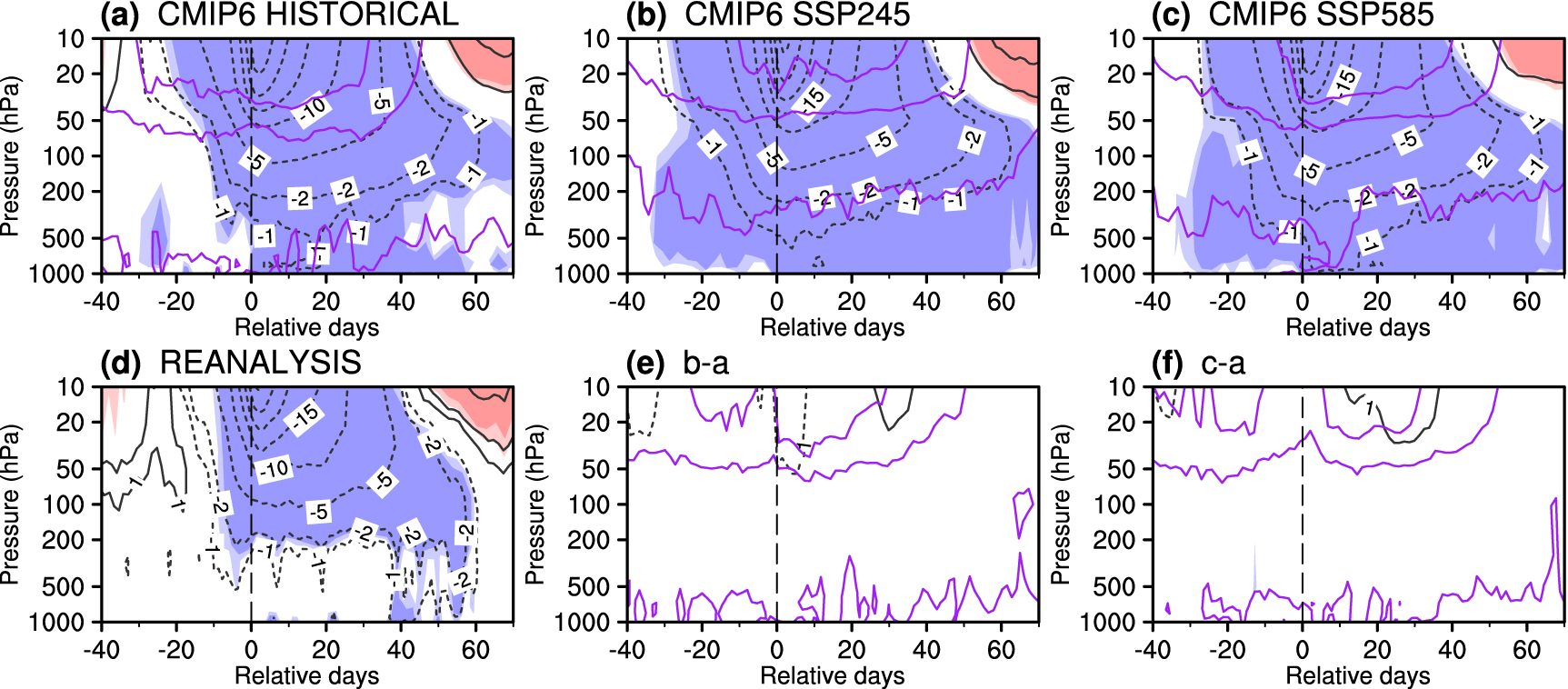
Projection of the stratosphere–troposphere coupling during SSWs by the CMIP6 MME is shown in figure 4. Although CMIP6 models more accurately simulate SSW frequency than CMIP5 models, the projected SSW evolution is nearly identical to CMIP5. As in the reanalysis (figure 4(d)), significant easterly anomalies develop from around day −20 and persist until day 40 at 10 hPa in the historical MME for CMIP6 (figure 4(a)). Significant near-surface responses form soon after the SSW onset due to the gradual downward propagation of the SSW signal. The SSP245 and SSP585 MMEs from CMIP6 (figures 4(b) and (c)) project a similar troposphere–stratosphere coupling during SSWs too, verified by the nearly zero difference between the future scenarios and the historical simulation (figures 4(e) and (f)). To summarize, both CMIP5 and CMIP6 do not project any significant change in the strength of the downward impact of SSWs in the future.
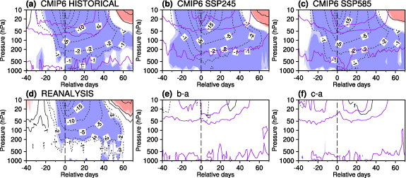
Figure 4. Composite evolutions of SSWs from day −40 to day 70 relative to the onset date of SSWs in (a) the historical simulation, (b) the SSP245 simulation, and (c) the SSP585 simulation. The reanalysis in (d) is shown as a reference for the evolution of SSWs in the present-day climate system, replicated from figure 3(d). Projected changes of the evolution of SSWs in (e) SSP245 and (f) SSP585 with respect to the historical simulation is shown in the last two plots. Contours are the zonal-mean zonal wind anomalies at 60° N from 1000 to 10 hPa, and light and dark shadings mark anomalies at the 90% and 95% confidence levels, respectively. All plots show the CMIP6 MME. The purple contours show the inter-model standard deviation of the wind anomalies or differences if applicable.
Download figure:
Standard image High-resolution image5. Projected change in the lifecycle of SSWs
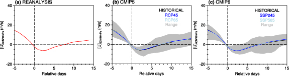
Another aspect of possible changes in SSWs is the persistency of circumpolar easterlies after the onset of SSWs. The average duration of circumpolar easterlies after an SSW can be used as a metric for the duration of a distorted or displaced stratospheric polar vortex, and it is conceivable that changes in, say, the concentration of greenhouse gases would impact radiative timescales in the stratosphere and hence alter the recovery of the vortex. Note that the persistency time of the circumpolar easterlies is much shorter than that of easterly anomalies during SSWs, but they are positively correlated among models and among events (not shown). The composite evolution of zonal-mean zonal winds at 10 hPa and 60° N is shown in figure 5 for the reanalysis and CMIP5/6. On average, the easterlies at 10 hPa develop on day 0 (by definition) and peak on day 3 in the reanalysis (figure 5(a)); from then on, the easterlies gradually decay and recover to westerlies on day 8. The historical MMEs from both CMIP5 and CMIP6 successfully simulate the SSW evolution in the historical runs (gray lines in figures 5(b) and (c)). Namely, the historical MMEs reproduce the easterlies from day 0 to day 8 and the maxima near day 3.
Figure 5. Life cycle of SSWs in (a) the reanalysis, (b) CMIP5, and (c) CMIP6. The zonal-mean zonal winds at 60° N and 10 hPa are shown from day −5 to day 15 relative to the onset date of SSWs. The historical, RCP45/SSP245, and RCP85/SSP585 simulations in (b), (c) are shown in gray, blue, and light blue, respectively. Only MME for CMIP5/6 is shown. No evident changes of life cycle of SSWs (i.e. persistence of easterlies and easterly maxima) are found from historical, to RCP45/SSP245, and then to RCP85/SSP585 simulations. The shading shows the inter-model value range.
Download figure:
Standard image High-resolution image
Based on the RCP45 and RCP85 MMEs from CMIP5 (blue and light blue lines in figure 5(b)), as well as the SSP245 and SSP585 MMEs from CMIP6 (figure 5(c)), the SSW evolution is projected not to change significantly. The evolution of SSWs in the historical, RCP45/SSP245, and RCP85/SSP585 simulations nearly overlays each other, implying a nearly identical evolution of SSWs in the future scenarios as in the historical simulations. Similarly, figures 3 and 4 indicate little change in the duration of easterly anomalies in the stratosphere following an SSW.
6. Summary and discussion
It is still unclear whether the statistical characteristics of SSWs will change in the future, with studies focusing on individual models or smaller model ensembles reaching opposite conclusions (Charlton-Perez et al 2008, Mclandress and Shepherd 2009, Bell et al 2010, Karpechko and Manzini 2012, Mitchell et al 2012, Kim et al 2017, Ayarzagüena et al 2018, 2020). This study focuses on this debate using the historical (as an estimate of the present-day climate system), RCP45/SSP245 (as a future projection in a moderate emissions scenario), and RCP85/SSP585 (as a future projection in a high emissions scenario) simulations from 54 state-of-the-art CMIP5/6 models. This larger dataset would allow us to more robustly identify future change in SSWs, if such changes were indeed projected to occur, than any previous study. The main findings are as follows.
- (a)Nearly 0.6 SSWs per year happen in the present-day climate system in the reanalysis, which is much better reproduced in the historical simulation from the CMIP6 MME than that from the CMIP5 MME. More CMIP5 models tend to underestimate the SSW frequency than CMIP6 models, but the sign (+) and amplitude of the change (∼0.05 more SSWs per year, insignificant) in the SSW frequency from historical simulations to RCP45/SSP245 and then to RCP85/SSP585 are consistently projected by CMIP5 and CMIP6 MMEs. Although more CMIP5/6 models show an increase in the SSW frequency, such a small increase is not significant.
- (b)There is little indication of a change in the timing of future SSWs among the winter months. However, CMIP5/6 models suffer from an apparent bias in the timing of SSWs in their historical simulations: too many SSWs occur in March and not enough in January. Such a bias in the seasonal distribution is not improved in CMIP6 when compared with CMIP5.
- (c)While the small increase in future SSWs when computed in all winter months is not statistically significant, a significant increase is simulated in individual months at the 5% level. However, the month with a significant increase in the SSW frequency is not consistent between CMIP5 and CMIP6. In other words, mid- (late-) winter SSWs are simulated to become more frequent by CMIP6 (CMIP5) in the future. The possible mechanisms that may lead to such an inconsistent increase among CMIP5/6 models in some wintertime months should be considered for future work.
- (d)The evolution of the NAM following SSWs is similar in reanalysis and in the CMIP5/6 historical experiments. Both exhibit significant easterly anomalies from around day −20 to day 40 at 10 hPa, with the signals gradually propagating downward. The near-surface responds instantly after the onset of SSWs in the historical experiments. Due to the large sample size in the CMIP5/6 ensembles, the SSW signals from the historical experiment are more significant than the reanalysis in a broader region. Both RCP45/SSP245 and RCP85/SSP585 from CMIP5/6 fail to project any significant change in the downward propagation of SSWs, implying the strength of stratosphere–troposphere coupling during SSWs will not change significantly relative to the present-day climate.
- (e)The average duration of SSWs is captured well by historical simulations of the CMIP5 and CMIP6 models. Specifically, the CMIP5 and CMIP6 MMEs successfully reproduce an 8 d persistent time of easterlies following onset of SSWs, and the easterly maxima near day 3 are also well simulated. Both RCP45/SSP245 and RCP85/SSP585 project a nearly identical composite evolution of SSWs, implying the lifecycle of SSWs will not change much relative to the present-day climate, even as greenhouse gas concentrations increase and radiative timescales change.
Overall, we find no significant changes in either the frequency, the seasonal distribution, the stratosphere–troposphere coupling, or the lifecycle of SSWs in two future scenarios relative to the present-day climate in historical simulations in the CMIP5/6 MMEs. That being said, mid- (late-) winter SSWs are projected to become more frequent by CMIP6 (CMIP5).
Our results are based on one definition of SSWs because of the large volume of data in the CMIP5/6 archive. While other definitions exist, the strongest events are typically captured by most or all definitions (Butler et al 2015). Nevertheless, it is conceivable that projections of the NAM response to SSWs might differ using other indices, as zonal wind at 60° N is a slightly poorer index of the NAM as compared to indices based on height (Baldwin and Thompson 2009). This possibility deserves further investigation in the future. Ayarzagüena et al (2020) find that the surface pressure response to SSWs is enhanced in the quadruple CO2 experiments relative to the preindustrial control experiments, and this study find little change in the stratosphere–troposphere coupling in the future. The experiments used in this study and Ayarzagüena et al (2020) are also different (RCPs/SSPs versus quadruple CO2). Moreover, this study adopts a larger model ensemble than Ayarzagüena et al (2020).
In addition, previous studies still debate on the possible surface impact of two SSW types (i.e. vortex displacement and split), so more work is required to further clarify this argument. The NAM strength is significantly different between vortex displacement and split SSWs based on the observational studies (Nakagawa and Yamazaki 2006, Mitchell et al 2013, Seviour et al 2013, 2016, O'Callaghan et al 2014), and the stronger surface impact of vortex splits than displacements might reflect the large intensity of the former, rather than the important role of the vortex morphology (Rao et al 2020). Future projections of the frequency of displacement and split SSWs is still unknown, and more analyses using other meteorological variables (especially height and temperature) need to be performed. However, our work provides a timely first insight into several aspects of little robust future change of SSWs projected by CMIP5 and CMIP6.
Acknowledgments
The authors thank the ESGF (https://esgf-node.llnl.gov/projects/esgf-llnl/) for their freely providing the CMIP5/6 simulations. All CMIP5/6 data used in this study are publicly available. The CMIP5/6 models (see tables 1 and 2) are developed by different agencies from different countries. This work was supported by the National Key R&D Program of China (2016YFA0602104) and the National Natural Science Foundation of China (41705024). CIG is also funded by the ISF-NSFC joint research program (3259/19) and the European Research Council starting grant under the European Union's Horizon 2020 research and innovation programme (677756).
Data availability statement
All data that support the findings of this study are included within the article (and any supplementary files).