

Abstract
Changes in rainfall affect drinking water, river and surface runoff, soil moisture, groundwater reserve, electricity generation, agriculture production and ultimately the economy of a country. Trends in rainfall, therefore, are important for examining the impact of climate change on water resources for its planning and management. Here, as analysed from 119 years of rainfall measurements at 16 different rain gauge stations across northeast India, a significant change in the rainfall pattern is evident after the year 1973, with a decreasing trend in rainfall of about 0.42 ± 0.024 mm dec−1. The wettest place of the world has shifted from Cherrapunji (CHE) to Mawsynram (MAW) (separated by 15 km) in recent decades, consistent with long-term rainfall changes in the region. The annual mean accumulated rainfall was about 12 550 mm at MAW and 11 963 mm at CHE for the period 1989–2010, as deduced from the available measurements at MAW. The changes in the Indian Ocean temperature have a profound effect on the rainfall in the region, and the contribution from the Arabian Sea temperature and moisture is remarkable in this respect, as analysed with a multivariate regression procedure for the period 1973–2019. The changes in land cover are another important aspect of this shift in rainfall pattern, as we find a noticeable reduction in vegetation area in northeast India in the past two decades, implying the human influence on recent climate change.
Export citation and abstract BibTeX RIS

Original content from this work may be used under the terms of the Creative Commons Attribution 4.0 license. Any further distribution of this work must maintain attribution to the author(s) and the title of the work, journal citation and DOI.
1. Introduction
Changes in regional climate represented by different meteorological conditions such as changes in temperature and precipitation are evident in observations and model simulations (IPCC special report 2018). Many of these changes are triggered by different anthropogenic activities such as greenhouse gas emissions and land use changes in the past century (e.g. Bindoff et al 2013). The contribution of anthropogenic and natural causes to changes in regional temperature and precipitation is very important in this context (e.g. Stott et al 2010, 2004, Balan Sarojini et al 2016, Varikoden et al 2019).
Observational evidence of human influence on global precipitation is challenged by the lack of long-term ground truth data sets and inadequate spatial coverage over different parts of the world, particularly over tropical land regions (Hegerl et al 2015, Balan Sarojini et al 2012). Yet there is growing evidence of human-induced changes in observed precipitation on global and latitudinal scales (e.g. Zhang et al 2007, Marvel and Bonfils 2013). Regionally, such increases or decreases in precipitation result in significant changes in water availability (Greve et al 2014, Padron et al 2020). For instance, a number of studies have shown increases in both the amount of rainfall received and its intensity across the United States and Canada in the last century. Groisman and Easterling (1994) found an increase of about 13% in annual precipitation in southern Canada and 4% in the United States during the last century (1891–1990). Zhang et al (2000) also reported that the annual precipitation has increased from 5% to 35% in southern Canada over the period 1900–1998. Karl and Knight (1998) reported that since 1910, precipitation has increased by 10% across the contiguous United States for the period 1910–1996. Similar changes in rainfall are also reported in different parts of Europe. The annual rainfall was found to have decreased slightly over Turkey, but significantly over the Black Sea and Mediterranean regions for the period 1930–1993 (Turkes 1996). A decreasing trend in annual, winter and autumn rainfall and an increasing trend in summer rainfall were observed over southern Italy over the period 1916–2000 (Caloiero et al 2011). The annual precipitation over Spain was estimated to have reduced during the period 1961–2006 (Rio et al 2011). In Serbia, winter and spring rainfall show decreasing trends, but positive trends in autumn rainfall during the period 1961–2009 (Luković et al 2014).
In addition, some of the studies carried out in Asia indicated that there are detectable changes in the rainfall in different regions. Herath and Ratnayake (2004) have analysed 30 year data from 1964 to 1993 and found a reduction in annual rainfall in the central mountainous region of Sri Lanka. Shahid (2011) reported a significant increase in annual and pre-monsoon rainfall together with an increase in heavy precipitation days, but a decrease in consecutive dry days in Bangladesh (1958–2007). Salma et al (2012) observed a decreasing trend of −1.18 mm dec−1 in rainfall from 1976 to 2005 over Pakistan. Mayowa et al (2015) showed a substantial increase in annual and monsoon rainfall, with an increase in the number of heavy rainfall days on the east coast of the Malaysian peninsula during the period 1971–2010. Analyses by Zhang et al (2005) found that the precipitation intensity was relatively weaker and maximum daily rainfall events were fewer over Southeast Asia from 1950 to 2003. Smith (2004) reported positive trends in annual rainfall due to increasing rainfall in summer over western, northern and central Australia during 1952–2002. However, they also report significant negative trends in winter rainfall over southwest Western Australia. Oguntunde et al (2011) found a sharp difference in rainfall between the periods 1931–1960 (increasing at 0.6 mm yr−1) and 1961–1990 (rapidly decreasing at 3.0 mm yr−1) in Nigeria. In tune with the changes in continental rainfall, large river basins on Earth also exhibit signatures of climate change by exposing large changes in precipitation. For example, the annual and seasonal rainfall in the Amazon basin shows negative trends for the past 70–80 years (Satyamurty et al 2010). Analyses of long-term and short-term trends of rainfall in the Nile River basin show positive trends in the equatorial regions of the basin for the period 1900–2004 (Onyutha et al 2016).
Apart from the recent changes in observed precipitation, model simulations such as the Coupled Model Intercomparision Project (CMIP) have also demonstrated similar changes in future rainfall across the continents. Akinsanola and Zhou (2019) report a statistically significant increase (decrease) in projected rainfall over the central eastern (western) Sahel sub-region for the global warming period (2045–2099). Chen et al (2013) project and discuss future changes in extreme rainfall events over China under Representative Concentration Pathway (RCP) 4.5 and RCP 8.5 scenarios for the period 2080–2099. Villarini et al (2013) show an increase in heavy rainfall over the central United States, which suggests a large increase in extreme rainfall mostly over the northern part of the country with much less over the Great Plains and the Gulf of Mexico for the periods 2006–2045 and 2046–2085. Salunke et al (2019) examined 28 CMIP5 model simulations of the climate of the Himalaya–Tibetan Plateau in the recent past (1975–2005). However, none of them was able to project the features of summer monsoon accurately. To understand the spatial and temporal variations of rainfall in the Malaysian peninsula, Noor et al (2019) used ensemble simulations of four CMIP5 models and projections for three periods 2010–2039, 2040–2069 and 2070–2099 in each RCP context. The projections showed increasing trends in rainfall for all scenarios. Jain et al (2019) used 28 models of CMIP5 for the historical period 1975–2005 of the Indian summer monsoon (ISM), but most models failed to capture the observed contribution ratio of convective and large-scale precipitation, and thus the monsoon rainfall.
The climate of India is governed by two prominent monsoon systems; the summer (southwest) and winter (northeast) monsoons. The ISM is associated with heavy rainfall during June–September and the winter monsoon during October–November. In India, agriculture relies on seasonal rainfall, and rice and tea are the two important crops that depend on ISM rainfall (ISMR). The monsoons play a key role in the growth of the country, as the amount of rainfall determines food production, electricity generation, and groundwater recharge and drinking water availability for most parts of India.
The northeast region of India consists of seven states covering a region from 22°05' to 29°30' N and from 87°55' to 97°24' E, with an area of about 262 230 km2. The region is about 1–7 km above sea level with an annual average rainfall of 2068 mm, mean temperature of 4 °C–30 °C, and relative humidity of about 70%–85%, depending on the region and season. The region is hilly, landlocked and falls into the subtropical climate classification. The land use statistics in the northeast show that about 64% of the land is within the forest area, about 30% under the Brahmaputra valley and the rest has steep slopes, hills and mountains (Basistha et al 2009). Although northeast India receives a good amount of rainfall during ISM, irregular and inhomogeneous rainfall have also been received in other seasons. Since agriculture is mainly rain fed, rice is the main crop in the region.
There have been significant changes in the land use and land cover (LULC) pattern in the northeast during the past three decades (Roy et al 2015). The anthropogenic activities have changed the traditional way of cultivation (i.e. shifting cultivation or Jhum cultivation) to cash crops, and there is sizeable deforestation (Leduc and Choudhury 2012) too. The primary source of income for the people is agriculture and horticulture during ISM. Agriculture and allied activities are considered to be the backbone of the economy of the region and are highly dependent on ISMR, where more than 60% of the crop area is under rain-fed agriculture (Ravindranath et al 2011). Therefore, accurate knowledge of the rainfall received and its temporal variability in the region are crucial for proper management of its land, industries, water resources and agriculture.
There are few studies available on the temperature and rainfall trends of the northeast region. For instance, Jain et al (2013) examined trends in rainfall for the period 1871–2008, and found no discernible change in the rainfall during the period. Jhajharia et al (2012) reported that measurements at four different regions of Assam showed no significant trend in rainfall for the period 1979–2000. Varikoden and Revadekar (2019) studied the rainfall trends in recent decades and found that the rainy days with high (low) intensity are increasing (decreasing) during ISM. However, measurements at a few stations showed decreasing trends in total rainfall in the pre-monsoon, monsoon and post-monsoon seasons. Also, a decreasing trend in annual rainfall was reported at 2.4 mm yr−1 in Agartala (AGT) (Tripura) during the period 1953–2000 (Jhajharia et al 2007, 2009). The aforementioned studies emphasize the necessity of studies in the northeast, as the existing analyses focus on one or two cities and for a shorter period. The region, which includes the wettest place on Earth, Cherrapunji (CHE), receives torrential rains in the monsoon seasons. Since northeast India is mostly hilly and is an extension of the Indo-Gangetic Plains, the region is highly sensitive to changes in regional and global climate. It has to be noted that the first signs of the effect of climate change will be evident for the extreme cases such as the rainfall at CHE. Henceforth, the analyses of rainfall over a century will give detailed information regarding the changes in rainfall induced by natural and anthropogenic forcing. Here, we use rainfall measurements from 16 rain gauge stations run by the India Meteorological Department (IMD) to study the trends and pattern change in rainfall in the northeast.
2. Data and methods
We have used daily and continuous rain gauge measurements from 16 stations, which are managed by IMD, spread across seven states of northeast India for the period 1901–2019 (Rajeevan and Bhate 2009). The stations considered for the analyses are Agartala (AGT), Aizwal (AIZ), Cherrapunji (CHE), Dibrugarh (DIB), Dhubri (DHU), Guwahati (GHY), Imphal (IMF), Itanagar (ITA), Jorhat (JOR), Kailashahar (KLS), North Lakhimpur (NLP), Pasighat (PGT), Shillong (SHG), Silchar (SLH) and Tezpur (TEZ). Although there are some other station measurements in the region, the data are not publicly available. In addition, we have selected the stations with the longest data records (i.e. more than a century of rainfall observations) for robust, meaningful and long-term trend analysis. The measurements from the available stations still well represent the northeast India region. The data presented are quality controlled and all caveats are considered for the analyses (e.g. Rajeevan et al 2006). However, the observations after 1970 are better calibrated and validated (e.g. Khouider et al 2020). We have also collected the available rainfall measurements from the Mawsynram (MAW) (25.28° N, 91.35° E) station, which are taken from the annual reports of the Meghalaya Planning Department. Since the MAW measurements are yearly averaged, they are not used for monthly and seasonal analyses as for the other stations. Figure 1 shows the measurement stations (top) and the measurements from the highest rainfall stations of CHE, SHG and SLH (middle panel). Measurements from MAW are presented in the bottom panel. Note that the measurements in the bottom panel are the annual accumulated rainfall. However, the measurements from other stations are daily averaged, as given by IMD, and are shown in figures 1 and S1 (available online at stacks.iop.org/ERL/16/024018/mmedia). Table S1 gives further details of the rainfall measurements. The satellite measurements from the Tropical Rainfall Measurement Mission (TRMM) and the reanalysis data ERA5 are also used for comparison with the surface measurements. To calculate the long-term trends in rainfall measurements, we have used simple linear regression (parametric) and its statistical significance obtained by Mann–Kendall test (non-parametric), as both methods are robust and widely accepted.
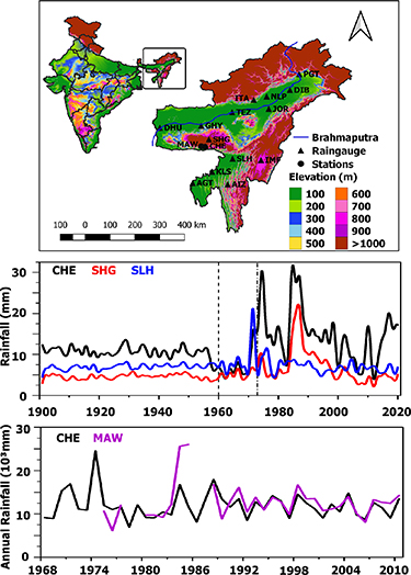
Figure 1. Rainfall measurements at the wettest place on Earth. Top: geographical maps of India and northeast India. Rainfall stations are also marked on the map. Middle: rainfall measurements at Cherrapunji (CHE), Shillong (SHG) and Silchar (SLH). Highest rainfall measurements in the northeast are observed at these stations. Bottom: rainfall measurements at the wettest places on Earth, CHE and MAW. Continuous measurements are only available only for the period 1989–2010 at MAW.
Download figure:
Standard image High-resolution imageSince there is an abrupt shift in the measurements before and after 1973, we have estimated the trends before (previous epoch: 1901–1972) and after (recent epoch: 1973–2019) this year. The turnaround year was selected after the statistical tests by applying linear regression, and by considering the previous analyses using rainfall measurements in the northeast. There are two distinct rainfall peaks in the rainfall time series around 1975 and 1985, and amplitude of the peak is higher in 1975. As illustrated in figures 1 and S1, different stations show the rainfall peaks in different years around 1975. When we consider the peak rainfall year as the starting point of trend analyses, that would corrupt the trend estimates. On the other hand, the previous analyses have demonstrated a climate shift around 1975/1976, but those studies did not estimate the trends in rainfall (Suhas et al 2008, Sabeerali et al 2012, Sahana et al 2015). Therefore, we have selected a year that is not inflicted with an abrupt shift in the rainfall as the turnaround year for the trend analyses. The statistical analyses are performed for different seasons; winter (January and February: JF), pre-monsoon (March, April and May: MAM), summer monsoon (June, July, August and September: JJAS), and post-monsoon (October, November and December: OND), and for the annual averaged measurements. Apart from these, we have also used another technique, multiple linear regression (MLR) developed by Nair et al (2018), to estimate the long-term trends in rainfall measurements and to understand the drivers of rainfall change in the region.
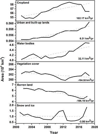
To monitor the changes of LULC at regular intervals, satellite remote sensing has been widely used (Roy et al 2015, Behera et al 2018). To decipher the anthropogenic influence of precipitation changes, we have exploited the Climate Change Initiative (CCI) merged LULC data for the period 1992–2018. These data have a resolution of 300 m, which is better than that of the Moderate Resolution Imaging Spectroradiometer (MODIS). In addition to the CCI data, we have also used the Landsat and MODIS satellite measurements for the assessment of LULC changes. Note that it has already been reported that there is a significant change in LULC in northeast India (Pielke et al 2011). Simple regression was used to find the rate of change for six different classes, i.e. vegetation, snow and ice, barren land, cropland, waterbodies and urban and built-up lands. Since the CCI (MODIS) observations start in 1992 (2001), that year is considered as the base period for LULC analyses for the period 1992–2018 (2001–2018).
2.1. Multivariate regression of rainfall
Several studies have shown the influence of many air, sea and land surface factors that control the rainfall changes in India across the seasons. Therefore, we have used an MLR that includes all known, but important and established drivers of Indian rainfall variability, as described in detail in Nair et al (2018). The major drivers include the sea surface temperature (SST) of the Indian, Atlantic and Pacific Oceans through various atmospheric and oceanic processes such as the Indian Ocean Dipole (IOD), Atlantic Zonal Mode (AZM) and El Niño and Southern Oscillation (ENSO; Seetha et al 2019). The north Indian Ocean surface temperatures are further modified by IOD events and are represented by the Dipole Mode Index (DMI; Ashok et al 2001). Therefore, the temperatures of the Arabian Sea (SSTA) and Bay of Bengal (SSTB) are also considered in the regression. The extratropical SSTs have an appreciable effect on the Indian monsoon and are represented by the Extratropical SST (ESST; Chattopadhyay et al 2015). The changes in equatorial winds (i.e. Equatorial Wind Index or EQWIN over the region 2.5° S–2.5° N and 60° E–90° E (Francis and Gadgil 2013) can influence the SST distribution in the tropical Indian Ocean as the Equatorial Indian Ocean Oscillation (EQUINOO) modulates the monsoon circulation, and is considered in the regression procedure. The connection between ENSO and Indian rainfall is well established, and is represented by the Multivariate ENSO Index (MEI), which is based on six atmospheric and oceanic variables of the Niño 3.4 region (5 °N–5° S and 170°–120 °W) of the eastern Pacific (Trenberth and Hoar 1997). The central Pacific ENSO is considered by taking the El Niño Modoki Index (EMI, Ashok et al 2007). The impact of the Atlantic Ocean surface temperatures on Indian rainfall is represented by two related processes, the Atlantic Multidecadal Oscillation (AMO, Goswami et al 2006) and AZM (Kucharski et al 2008). The index corresponding to AZM is computed from the SST anomaly over 3° S–3° N and 20°–0° W, but the region 0°–60° N and 75°–7.5° W for AMO. In addition, a new Index is introduced in this study, which is the normalized difference vegetation index (NDVI) to represent the changes in LULC and vegetation in the northeast. The NDVI data are taken from the Landsat measurements. The MLR is then constructed for this study in the following form:
where R is the rainfall, C(t) is the linear trend,  is the residual, t is the year and A is constant and is considered as 1. The terms with C as the prefix represent the corresponding regression coefficients (e.g. CMEI is the regression coefficient of time series of MEI, which determines the contribution of the process represented by MEI when the other variables are kept constant in the regression procedure). The trend is considered as statistically significant when the value is greater than twice its standard deviation (i.e. in the 95% confidence level) here. The proxies and residuals are roughly normally distributed and the proxies are not auto-correlated. Further discussion on the model and its performance is given in Nair et al (2018).
3. Results and discussion
3.1. Spatial and temporal distribution of rainfall
In general, the rainfall starts in pre-monsoon by March and peaks during ISM from June–September at all stations, and figure 2 shows the monthly distribution of rainfall at different stations in the northeast. However, there is small spatial inhomogeneity in the peak rainfall, as seven stations show the peak rainfall in June and the remaining in July. The rainfall distribution is about 10 mm in April and peaks to 15–20 mm in June–July, depending on the stations. The CHE station is an exception to this, as it shows about 5 mm in March, about 15 mm in May, peaks to 30 mm in June, and a gradual decrease thereafter. Therefore, it exhibits heavy rainfall throughout the year, which makes the region the wettest place on Earth. As also mentioned in section 2, the time series data of rainfall at each station show a distinct difference in annual rainfall after the mid-1970s (figures 1 and S1) and thus, we have divided our analyses into before and after the year 1973. This apparent shift in the regional climate was also reported in earlier studies (Basistha et al 2009, Deka et al 2013, Goyal 2014) and henceforth, 1973 is taken as the turning year for the recent epoch. The monthly distribution of rainfall is similar at all stations (figure 2). Nevertheless, the rainfall exhibits a significant decrease in the recent epoch at most stations, except for DHU and JOR. It is also interesting to note the change in peak rainfall period in some stations in the recent epoch (1973–2019) compared to the previous epoch, and is explicit at CHE and SHG, where the peak rainfall occurs a month later than in the previous epoch. This demonstrates the spatial and temporal changes in rainfall in northeast India, including the wettest place on Earth.

Figure 2. Spatial inhomogeneity and temporal changes in climatological rainfall at the wettest place on Earth and other locations. Monthly average rainfall computed for three different time periods at 15 stations located in northeast India. Station measurements considered for the analyses are Agartala (AGT), Aizwal (AIZ), Cherrapunji (CHE), Dibrugarh (DIB), Dhubri (DHU), Guwahati (GHY), Imphal (IMF), Itanagar (ITA), Jorhat (JOR), Kailashahar (KLS), North Lakhimpur (NLP), Pasighat (PGT), Shillong (SHG), Silchar (SLH) and Tezpur (TEZ). Spatial inhomogeneity in the monsoon onset and peak rainfall period is evident in the illustrations. Vertical dotted lines at June and September represent the peak rainfall period (June–September).
Download figure:
Standard image High-resolution imageThe northeast region experiences distinct seasonal variation in rainfall. Figure 3 shows the average (of all stations) rainfall received in the region in different seasons and each year. The values are computed for each season in a year and are represented by the year of the corresponding season. The winter rainfall shows the lowest among the seasons, about 1 mm, and the rainfall increased to 2 mm in 1917 and 1998, although in many years it was close to zero, such as in 1979 and 1999. The monsoon rainfall is also lower and almost 1 mm higher than that of winter, as the average rainfall in the season is about 2 mm. In some years, the rainfall amounts to 5 mm, as in 1986 and 3 mm in 1928, but hardly any in 1935 and 2015. Pre-monsoon and monsoon are the rainy seasons of northeast India. Average rainfall of about 6 mm during pre-monsoon and twice of that during monsoon are observed there with large inter-annual variability. The pre-monsoon showers show inter-annual changes of between 4 and 10 mm, but some extreme rainfall events such as 2 mm in 1961, 10.5 mm in 1930, 1977 and 2017 are also observed. The highest annual pre-monsoon rainfall occurred in 2010, about 11 mm. The monsoon rainfall oscillates between 9 and 22 mm, and the rainfall scales about 13 mm in most years. The highest monsoon rainfall in the region was recorded in 1974, about 22 mm, and the lowest rainfall was registered in 1963, about 8.5 mm. The amount of annual average rainfall received in the region coincides with the pre-monsoon rainfall, which is about half of the rain received during ISM, about 5–10 mm.

Figure 3. Temporal evolution of seasonal rainfall in northeast India during the past century. Seasonal and annual rainfall averaged for 15 stations in northeast India from 1901–2019. Vertical dashed line indicates the year 1973.
Download figure:
Standard image High-resolution imageLarge variability is observed at the stations that experience high rainfall, such as at CHE, SHG, and SLH (figure 1), but little inter-annual variability is found at KLS, TEZ, GHY and IMF. Previous analyses suggest that the abrupt increase in rainfall after the 1970s in the CHE station is due to the anomalous anticyclonic circulation over central India and the northern Bay of Bengal at 200 and 850 hPa levels. The positive OLR anomaly and moisture divergence anomalies show suppression of convection over western India. The convergence of anomalous moisture flux over northeast India coincides well with active convection over northeast India, which drives above normal rainfall there (e.g. Murata et al 2007).
3.2. Long-term trends in rainfall (1901–2019)
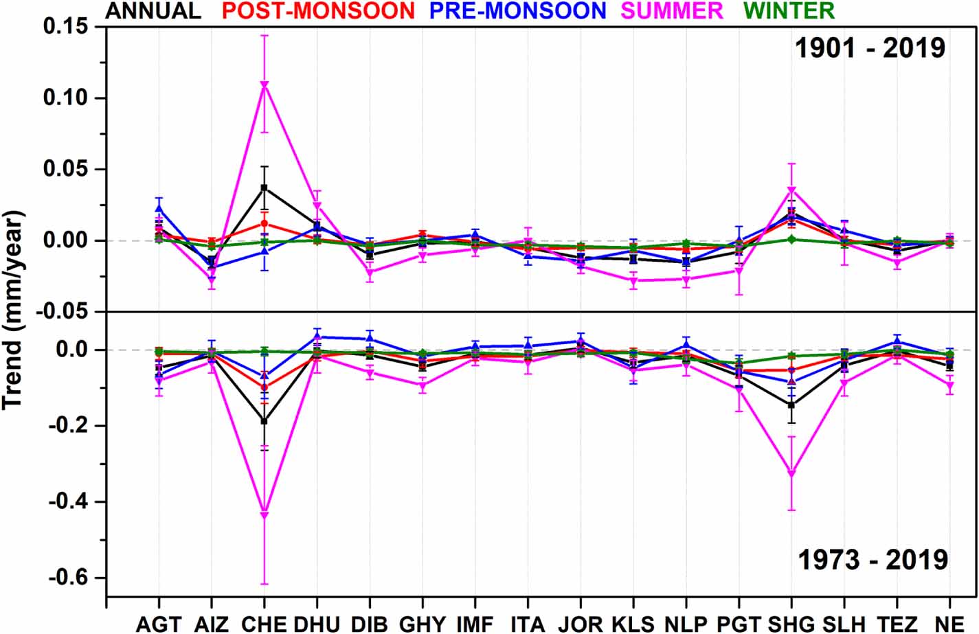
In general, most stations show the largest decreasing trend in rainfall in summer and the lowest in winter (figure 4, table 1). The decreasing trend in the southwest monsoon is about 0.001–0.280 mm dec−1, and is largest at KLS, about 0.28 mm dec−1. Six stations show statistically significant negative trends in the rainfall, i.e. at AIZ, DIB, JOR, KLS, NLP and TEZ. Although not statistically significant, negative trends are estimated at GHY, IMF, ITA, PGT and SLH. However, statistically significant positive trends are observed at CHE, DHU and SHG, but are insignificant at AGT. A clear reduction in rainfall is evident at most stations since the late 1970s (figures 2 and S2). Nonetheless, the estimated trends at CHE and SHG must be interpreted carefully as there is a steep decrease in rainfall at both stations since mid-1980. Detailed trend analyses for the period 1973–2019 are also shown in figure 4 (bottom) and table S2.

Figure 4. Trends in rainfall at the wettest place on Earth and its surrounding regions. Top: trends in rainfall at different stations in northeast India for the period 1901–2019. Bottom: trends estimated for the recent epoch (1973–2019). Station measurements considered for the analyses are Agartala (AGT), Aizwal (AIZ), Cherrapunji (CHE), Dibrugarh (DIB), Dhubri (DHU), Guwahati (GHY), Imphal (IMF), Itanagar (ITA), Jorhat (JOR), Kailashahar (KLS), North Lakhimpur (NLP), Pasighat (PGT), Shillong (SHG), Silchar (SLH) and Tezpur (TEZ). Error bars represent twice the standard deviation from the mean. Trends computed for CHE (CHE is divided by a factor of 2.0 to fit into the scale of other estimates).
Download figure:
Standard image High-resolution imageTable 1. Trends in rainfall at the wettest place on Earth and nearby stations. The trend in annual average, winter, pre-monsoon, monsoon and post-monsoon rainfall time series (1901–2019). Values shown in 'bold' indicate the confidence level at 5%. Trends estimated for the recent epoch (1973–2019) are shown in table S2.
| Station | Annual Average | Winter | Pre-monsoon | Monsoon | Post-monsoon |
|---|---|---|---|---|---|
| mm dec−1 | mm dec−1 | mm dec−1 | mm dec−1 | mm dec−1 | |
| 1. Agartala (AGT) | +0.095 ± 0.081 | +0.007 ± 0.032 | +0.223 ± 0.161 | +0.080 ± 0.158 | +0.043 ± 0.069 |
| 2. Aizwal (AIZ) | −0.15 ± 0.071 | −0.040 ± 0.042 | −0.190 ± 0.138 | −0.270 ± 0.131 | −0.01 ± 0.06 |
| 3. Cherrapunji (CHE) | +0.371 ± 0.285 | −0.01 ± 0.049 | −0.08 ± 0.247 | +1.098 ± 0.673 | +0.119 ± 0.154 |
| 4. Dhubri (DHU) | +0.106 ± 0.078 | −0.001 ± 0.027 | +0.089 ± 0.119 | +0.247 ± 0.197 | +0.008 ± 0.06 |
| 5. Dibrugarh (DIB) | −0.10 ± 0.061 | −0.040 ± 0.039 | −0.03 ± 0.105 | −0.220 ± 0.139 | −0.03 ± 0.048 |
| 6. Guwahati (GHY) | −0.020 ± 0.048 | −0.005 ± 0.023 | −0.001 ± 0.063 | −0.10 ± 0.103 | +0.044 ± 0.059 |
| 7. Imphal (IMF) | −0.010 ± 0.041 | −0.030 ± 0.032 | +0.04 ± 0.07 | −0.06 ± 0.09 | −0.01 ± 0.055 |
| 8. Itanagar (ITA) | −0.05 ± 0.074 | −0.03 ± 0.039 | −0.11 ± 0.13 | −0.001 ± 0.173 | −0.060 ± 0.064 |
| 9. Jorhat (JOR) | −0.12 ± 0.047 | −0.040 ± 0.031 | −0.14 ± 0.10 | −0.180 ± 0.092 | −0.050 ± 0.041 |
| 10. Kailashahar (KLS) | −0.13 ± 0.064 | −0.050 ± 0.039 | −0.07 ± 0.161 | −0.280 ± 0.122 | −0.050 ± 0.062 |
| 11. North Lakhimpur (NLP) | −0.15 ± 0.058 | −0.02 ± 0.042 | −0.150 ± 0.113 | −0.270 ± 0.117 | −0.060 ± 0.042 |
| 12. Pasighat (PGT) | −0.08 ± 0.15 | −0.04 ± 0.066 | +0.004 ± 0.19 | −0.21 ± 0.335 | −0.04 ± 0.084 |
| 13. Shillong (SHG) | +0.204 ± 0.164 | +0.009 ± 0.028 | +0.167 ± 0.126 | +0.364 ± 0.352 | +0.155 ± 0.113 |
| 14. Silchar (SLH) | +0.006 ± 0.126 | −0.002 ± 0.0051 | +0.073 ± 0.134 | −0.02 ± 0.289 | −0.006 ± 0.063 |
| 15. Tezpur (TEZ) | −0.070 ± 0.047 | −0.0001 ± 0.0036 | −0.03 ± 0.082 | −0.150 ± 0.105 | −0.03 ± 0.039 |
In winter, insignificant positive trends are found at AGT and SHG, and insignificant negative trends are estimated for AIZ, CHE, DHU, GHY, IMF, ITA, NLP, PGT, SLH and TEZ. Statistically significant negative trends are observed at the remaining three stations. Similar to winter rainfall, the pre-monsoon data show statistically significant positive trends at AGT and SHG in 1901–2019. On the other hand, AIZ, JOR and NLP show statistically significant negative trends, although CHE, DIB, GHY, ITA, KLS and TEZ show statistically insignificant negative trends. The monsoon (June–September) rainfall shows increasing trends at AGT, CHE, DHU and SHG, and except for AGT the remaining stations show statistically significant rainfall trends. On the other hand, decreasing trends are observed at AIZ, DIB, JOR, KLS, NLP and TEZ, which are statistically significant, while the trends at the remaining stations are insignificant. In the case of post-monsoon rainfall, ten stations exhibit a decreasing trend, for which JOR and NLP show statistically significant trends. In contrast, AGT, CHE, DHU, GHY and SHG show positive trends, in which the SHG measurements are statistically significant.
3.3. Rainfall changes during the recent epoch (1973–2019)
The annual mean rainfall for the period 1973–2019 shows decreasing trends of about 0.42 mm dec−1 and are statistically significant, along with seven other stations, i.e. AGT, CHE, GHY, KLS, PGT, SHG and SLH. The winter rainfall is decreasing in the northeast at all stations (0.11 mm dec−1, from the linear trends calculated for both periods, as shown in the figure 4 bottom panel and table S3) and this reduction in rainfall is statistically significant at NLP, PGT and SHG. In pre-monsoon (March–May), eight stations show a decreasing trend in rainfall in which only one station shows a statistically significant trend, i.e. at SHG. On the other hand, seven stations show an increasing trend in rainfall, but none is statistically significant. The rainfall during the pre-monsoon season, throughout the study area, shows a statistically insignificant decreasing trend (table S3).
The analyses are again cross-checked with the ERA5 rainfall data by applying the same trend detection method (table S4). As discussed, most stations show decreasing trends in rainfall across the seasons, where the trends in winter, pre-monsoon and post-monsoon are dominated by decreasing rainfall at most stations. The trend values are also comparable, such as the estimated annual averaged rainfall trends of −0.14 ± 0.25 mm dec−1 at KLS and −0.13 ± 0.68 mm dec−1 at CHE. It is interesting to note the negative trends estimated for the CHE and SHG data (0.1–0.3 mm dec−1), which are consistent with the surface measurements, implying that the rainfall is decreasing at the wettest place on Earth in all seasons. The negative trends shown at PGT and DIB are statistically significant, and are around 0.62 mm dec−1. Nonetheless, the trends at DHU, GHY, IMF and ITA show positive values as the rainfall received in each season at these stations is higher than that of other stations.
There are two distinct peaks in the observed rainfall measurements at CHE around the mid-1970s and mid-1980s for the period 1901–2019. This is clearly illustrated in figures 1 and S2. The trend estimated for the first epoch has a part of one of these peaks and the data up to 1950 have no clear temporal trends. Therefore, the trend estimated for the first epoch, which is weighted by the measurements during the period 1950–1972, is positive. On the other hand, the trend estimates in the second epoch include a part of the peak of mid-1970, the high rainfall in the mid-1980s, and the lowest rainfall ever recorded at CHE in the late 2000s. These make the trend value negative for the recent decade. This is the reason that we performed a test on the turnaround period for trend estimates, as the initial and end year measurements are very important and would influence the linear trend estimates.
In brief, ISMR at most stations shows a decreasing trend for the period 1973–2019. The analyses show a reduction in rainfall at all stations, in which seven are statistically significant. These analyses clearly demonstrate that the rainfall is decreasing during the recent epoch in northeast India. The decrease in rainfall is also evident at the wettest place on Earth (CHE) and its nearby station (SHG), and both stations are situated at higher elevations (figure 1 and table S1). It is evident from our analysis that northeast India receives a smaller amount of rainfall during ISM in this epoch compared to the previous epoch. This is also consistent with the analysis for the period of 119 years (1901–2019) over the entire northeast region that showed an insignificant decreasing trend of 0.001 mm dec−1. In post-monsoon, all stations show negative trends in rainfall and are significant at two stations, i.e. CHE and PGT. The inter-annual variability is comparatively smaller for the post-monsoon rainfall at all stations (figure 3).
3.4. Drivers of rainfall change in northeast India
To further assess the estimated trends, we have used another method of trend analysis, the MLR, as discussed in section 2.1. The method also indicates the contribution of different remote and local forces to rainfall change in northeast India. The analyses of 119 years of rainfall data show that there is a significant reduction in the rainfall received in all seasons in both epochs. The decrease in rainfall over the period on the wettest place on Earth is even more evident and alarming. In all seasons, the rainfall shows a substantial reduction, except in pre-monsoon. The smallest trend is observed in pre-monsoon and post-monsoon, around −0.18 mm dec−1, and the largest in the summer monsoon, about −0.785 mm dec−1 (table S5). The pre-monsoon trends show small positive values, implying the changes in rainfall as it is normally infrequent and very light in this season. However, trends in this season also show signatures of significant change. We did a separate analysis for the wettest place, CHE, where all seasons, except pre-monsoon, show a substantial reduction in rainfall in the recent epoch (1973–2019). The estimated trends for the northeast and CHE are statistically significant in all seasons and for the annual averaged data, except for the pre-monsoon showers, where the trends show insignificant positive values. The magnitude of decreasing trends is several times the average for the whole northeast (e.g. seven fold in post-monsoon, about −0.8 ± 0.3 mm dec−1) and are significant too; showing the rapid changes in the rainfall and its intensity in the region. The change in rainfall pattern also moved the rainfall intensity and frequency to further west of CHE to MAW, which makes the latter the wettest place on Earth.
These results are also confirmed by the analyses with annual accumulated rainfall at CHE and MAW (shown in the figure 1 bottom panel). The analyses show that the average rainfall at CHE is about 11 963 ± 2346 mm (i.e. average ± standard deviation) and MAW is about 12 550 ± 2321 mm for the period 1989–2010. The linear trends computed for the same period also show a larger decrease of about 27 ± 39 mm yr−1 at CHE and 6.9 ± 73 mm yr−1 at MAW. The highest ever rainfall in the northeast was measured at MAW, about 26 000 mm in 1985–1986. These rainfall measurements also reveal that the wettest place on Earth moved from CHE to MAW by the late 1970s. Some of the expected signatures of climate change are indeed the changes in regional rainfall pattern and warming of the world oceans. Henceforth, we explore further to understand the causes of the significant changes in rainfall that are clearly visible in northeast India.
3.5. Contributory factors to inter-annual variability
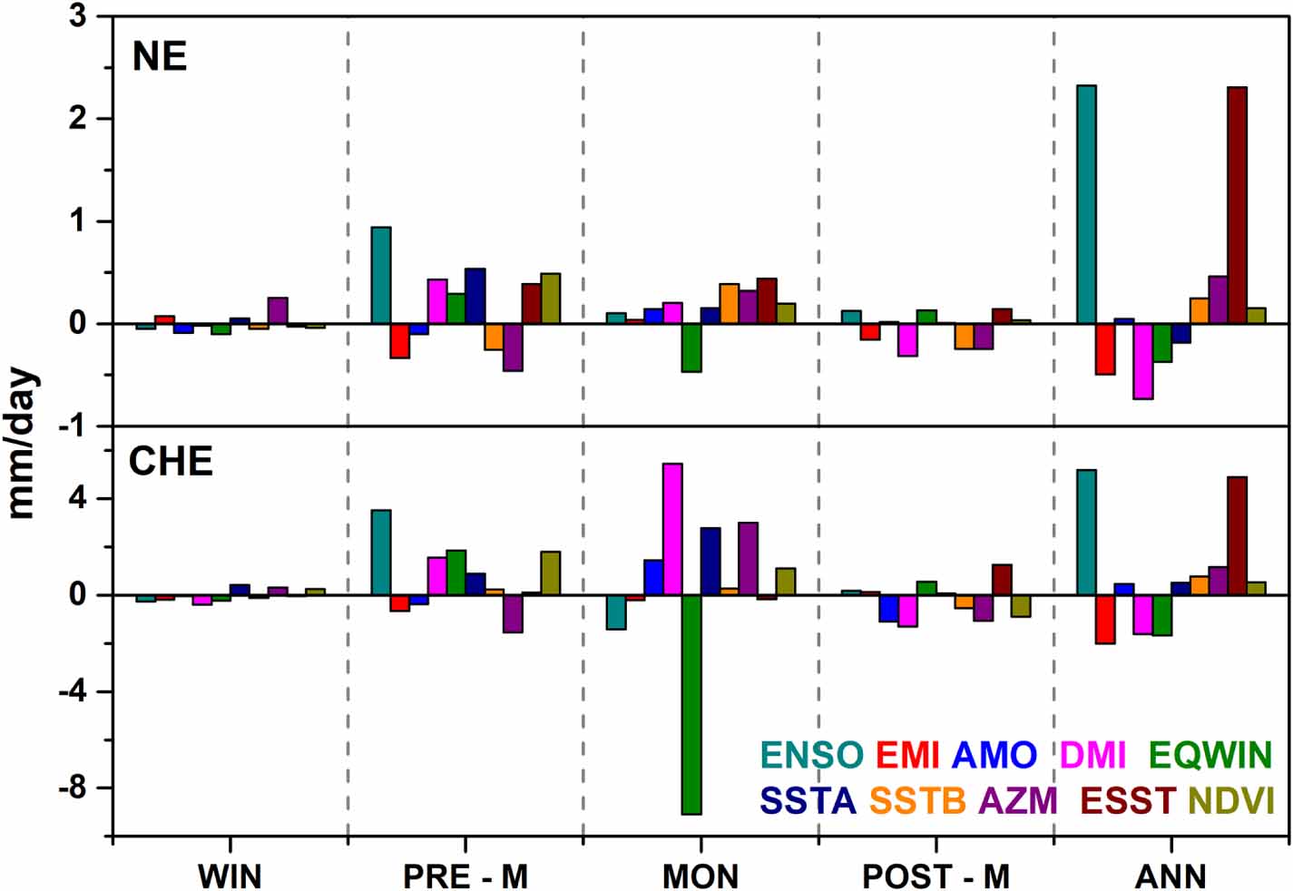
We analysed the contributory factors to the rainfall variability in northeast, computed using the MLR and are illustrated by figure 4 (top: northeast, bottom: CHE). The winter rainfall is about 1 mm on average and the contributions from different factors are also lowest in that season. The contribution of different factors is smaller in the post-monsoon season and are mostly negative, but the ENSO and equatorial winds dominate there, and are less than 0.5 mm of rain. In pre-monsoon, most factors favour rainfall and contribute to 0.5–1 mm and the contribution from ENSO is the largest among the factors. The changes in the SST of Arabian Sea and the equatorial Indian Ocean (i.e. DMI and ESST) contribute to the rainfall in pre-monsoon. In addition, the analyses show that the NDVI or the vegetation also plays a significant role in rainfall during pre-monsoon due to healthy leaf senescence there, about 0.7 mm. During monsoon, all factors except equatorial winds (EQWIN) contribute positively to the rainfall, which is about −1.0 mm by EQWIN. The other factors contribute up to 0.8 mm of rain, and the contribution of the equatorial Bay of Bengal and Atlantic SST is noticeable. The NDVI also contributes about 0.4 mm of rain in this season, which is greater than that of four other contributory factors.
The regression with annual averaged rainfall data shows appreciable contribution from ENSO and equatorial ocean temperatures (ESST), about 2.2 mm. The north Atlantic and Bay of Bengal surface temperatures, and vegetation cover contribute about 0.2–0.4 mm. However, as far as the changes in temperatures of the north Indian Ocean are concerned, SSTB has a greater influence than SSTA and its contribution is about −0.5 mm yr−1. The influence of equatorial winds and Arabian Sea is very limited and their contributions to rainfall are negative. This suggests that the changes in moisture transport from the Arabian Sea do not significantly affect the southwest monsoon rainfall in the northeast compared to that from the Bay of Bengal, consistent with the analyses of Nair et al (2018).
Nevertheless, there is a spatial inhomogeneity in the contribution of different factors of rainfall change. For instance, as the rainfall in CHE is the highest in the world, henceforth, proportionately higher values of contributions from different factors are estimated there. Since monsoon rains are highest among the seasons, the largest contribution is found during this season and mostly, the Atlantic and Indian Ocean temperatures decide the amount of rainfall received in this season, about 3–5.5 mm. The changes in vegetation also have a key role in the variability of rainfall there, about 1.5 mm. Conversely, the strength of equatorial winds has a greater role in suppressing the rainfall and its contribution amounts to −8 mm, the largest among the contributory factors. The annual rainfall shows the contribution mostly from the Pacific and equatorial Indian Ocean surface temperature changes. Since vegetation or land cover changes play a predominant role in rainfall in the northeast and CHE regions, we further examine this aspect in detail in the next section using LULC analyses.
3.6. LULC changes in northeast India
There is a significant change in LULC in recent decades in northeast India and the changes are mostly in the forest cover and vegetation in the region. Although the published records may not show the up-to-date extent of deforestation, satellite measurements can pinpoint the actual deforestation and all types of LULC. Therefore, we have used satellite observations for monitoring the temporal changes in LULC in the region. During the past few decades, the LULC of India was changed substantially due to the increase in population from 1951 (361 million) to 2011 (1221 million as per the latest census report of 2011) and due to development activities (Moulds et al 2018). Northeast India has the highest vegetation cover in India and includes 18 biodiversity hotspots of the world, indicating the importance of the region in terms of its greenery and climate change sensitivity. Population growth demands more food production and infrastructure development, and has changed the LULC of the region. Forest cover is the most exposed vegetation type to anthropogenic activities such as the conversion of forestland to mining, agriculture, urban area expansion and railroad construction (Lele and Joshi 2009, Chitale and Behera 2014). Therefore, we have done an analysis on the LULC change in northeast using satellite measurements and the results are shown in figure 5 and table S3.

Figure 5. Contribution of prominent regional and global climate factors to the rainfall in northeast India and the wettest place on Earth. Contribution of different indices to rainfall in the northeast region (top panel) and for Cherrapunji (bottom panel) during winter (WIN), pre-monsoon (PRE-M), monsoon (MON) and post-monsoon (POST-M) for the recent epoch (1973–2019). Rainfall is measured in mm d−1. Factors represented in the multivariate regression to estimate the individual contribution to rainfall are ENSO (El Niño and Southern Oscillation), EMI (El Niño Modoki Index), AMO (Atlantic Multidecadal Oscillation), DMI (Dipole Mode Index), EQWIN (equatorial winds associated with Equatorial Indian Ocean Oscillation—EQUINOO), SSTA (Arabian Sea surface temperature), SSTB (Bay of Bengal SST), AZM (Atlantic Zonal Mode), ESST is Extratropical SST, and NDVI (normalized difference vegetation index).
Download figure:
Standard image High-resolution imageOur analysis (figure 6) shows noticeable reductions in vegetation (−104.5 km2 yr−1), barren land (−106.1 km2 yr−1) and snow and ice (−3.9 km2 yr−1), but significant increases in cropland (182.1 km2 yr−1), water bodies (32.1 km2 yr−1), urban and built-up lands (0.3 km2 yr−1) during the period 2001–2018. The change in percentage area reveals that the waterbodies, urban regions and built-up areas are continuously increasing from the reference year of 2001. However, the decrease in vegetation cover and increase in the areas of cropland are observed from the year 2006 onwards, implying the conversion of forestlands and vegetation cover to croplands. This is also the first step of the urbanization practice, as forest or vegetated areas are converted to croplands and then those lands will be eventually altered to urban settings. The changes in snow cover over the years can be linked to the slow warming in the region, which also increased the barren lands at higher elevations and led to the expansion of waterbodies. The increase in barren lands in the lower elevation areas exhibits its use for urban conversions. It has to be noted that the Indian government has launched a number of socio-economic schemes to enhance the lives of people there, such as the Mahatma Gandhi National Rural Employment Guarantee Scheme, Joint Forest Management, Japan International Cooperation Agency and Indo–German Development Cooperation Project. A number of check dams of small and medium size watersheds have also been constructed as a part of these schemes, and are the other reasons for the small increase in waterbodies in the past two decades (e.g. Behera et al 2018).
Figure 6. Temporal changes in the LULC in northeast India. Changes in the LULC compared to the base year 2001 in northeast India.
Download figure:
Standard image High-resolution image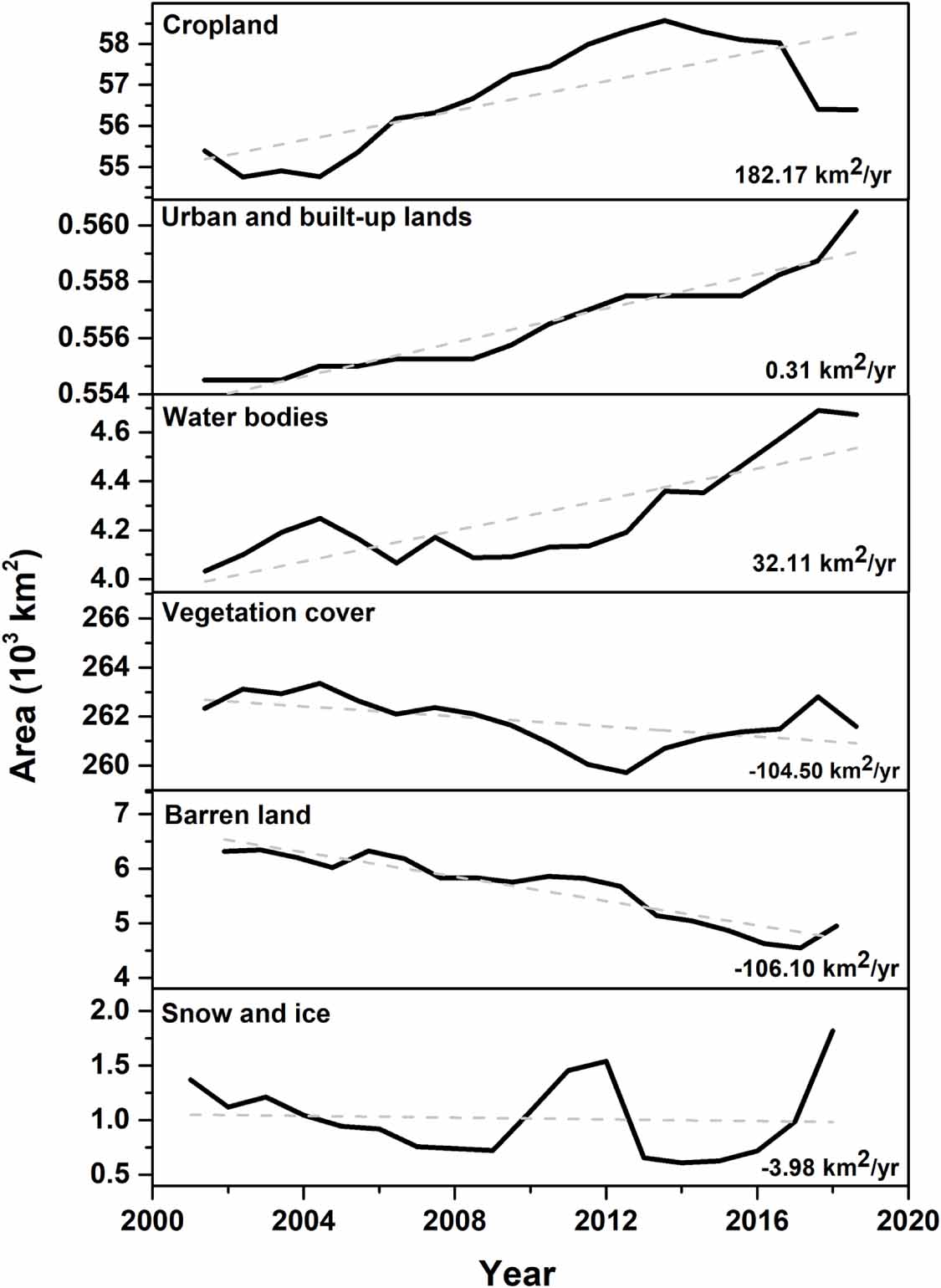
We also used the CCI data to investigate the MODIS results, which are shown in figure S2 and table S7. Both data show similar changes for most LULC components for the overlapping time period (2001–2018, red trend line in figure S2). However, there is a small difference in snow and ice area analyses, as the MODIS data show a significant decrease in its area, but no detectable decrease is found with the CCI data. Although the waterbodies show a decreasing trend in CCI data, the MODIS data show an increasing trend in their area since 2001. Yet, the area of waterbodies shows an increasing trend from 2005 onwards; confirming the positive trends estimated with the MODIS data. Therefore, both data sets reveal similar changes in most LULC components and suggest significant alterations in LULC in northeast India. Nevertheless, these results also show the uncertainties in different land surface variables of LULC in different satellite data. The changes in LULC have a negative impact on the precipitation through the modification of temperature by evapotranspiration in the region, as shown by the negative trends in rainfall of CHE and SHG, which are the heavy rainfall regions in the northeast and on Earth. Note that the climate change signatures will be first evident for the extreme cases, such as the rainfall received at the then wettest place in the world, and as such, CHE and is clearly exposed in our analyses.
4. Conclusion
We find that the rainfall starts in pre-monsoon by March and peaks during the ISM from June–September in northeast India, using 119 years of daily rain gauge measurements during 1901–2019. The amount of pre-monsoon rainfall is about half of that which occurs during monsoon (e.g. 10 mm). Most stations in northeast India show negative trends in rainfall, with the largest negative trends in ISM and the smallest in winter. The decreasing trend in ISM is about 0.001–0.280 mm dec−1, and is largest at the station KLS, about 0.280 mm dec−1 in the past 119 years. The change in rainfall at CHE, the wettest place on Earth, demonstrates the spatial changes in rainfall with time. The spatial pattern change in the rainfall in the region during the recent epoch (1973–2019) is also the reason for the observed shift of the wettest place from CHE to MAW. Indian Ocean temperatures play a dominant role in this pattern change, as demonstrated by the remarkable contribution of the Arabian Sea SST and moisture to the regional rainfall for the period 1973–2019. The drastic changes in forest and vegetation in northeast India due to human activities also influence the rainfall pattern in the region, as the changes in vegetation highly correlate with the decreasing trends in rainfall in recent decades. These analyses clearly demonstrate the anthropogenic influence on rainfall changes in the region, and the impact of developmental activities and deforestation on regional climate.
Acknowledgments
We thank the Head CORAL and the Director, Indian Institute of Technology Kharagpur (IIT Kgp), the Sponsored Research and Industrial Consultancy of IIT Kgp (Project CMI/SRIC), the Department of Science and Technology (DST) of the Ministry of Human Resource Development, the National Centre for Ocean Information Services Hyderabad of the Ministry of Earth Science (O-MASCOT project) and the Naval research Board of Defence Research and Development Organisation for facilitating and funding the study (OEP-NRB project). SR, SM, and PK acknowledge the support from MHRD and IIT KGP. The MODIS data sets were acquired from the Level-1 and Atmosphere Archive and Distribution System (LAADS) Distributed Active Archive Center (DAAC), located in the Goddard Space Flight Center in Greenbelt, Maryland (https://ladsweb.nascom.nasa.gov/). HV is grateful to the Director, Indian Institute of Tropical Meteorology, Pune, for the support. PJN is grateful to Head CORAL, and DST New Delhi for the WOS-A/KIRAN woman scientist fellowship. The authors gratefully acknowledge the India Meteorological Department, Pune, India, for providing rainfall data, and NASA and NOAA for climate indices for the MLR analyses.
Data availability
The rainfall data are available from the India Meteorological Department (IMD). The TRMM data are taken from (http://daac.gsfc.nasa.gov/precipitation/TRMM_README/TRMM_3B43_readme.shtml). The ENSO data are taken from (www.esrl.noaa.gov/psd/data/climateindices/list/), The AMO data are from (www.esrl.noaa.gov/psd/data/timeseries/AMO/), the DMI data are taken from the HadISST version 1.1 available at (www.esrl.noaa.gov/psd/gcos_wgsp/Timeseries/DMI/index.html) and the EQWIN data are from the Indian National Centre for Ocean Information Services. The Indices are calculated by PJN, and are available upon request. For LULC analysis, we have used MODIS Land Cover Type Product (MCD12Q1), which has 500 m spatial resolution at annual time steps from 2001–2018 and these data sets are freely available on registration within the sites (https://lpdaac.usgs.gov/products/mcd12q1v006/). ESA. Land Cover CCI Product User Guide Version 2. Tech. Rep. (2017). Available at: maps.elie.ucl.acbe/CCI/viewer/download/ESACCI-LC-Ph2-PUGv2_2.0.pdf
The data that support the findings of this study are available upon reasonable request from the authors.
Author contributions
JK conceived the idea and designed the research. JK, HV, SM, BBS and PS further developed the research. SM, HV, PK, SR and PJN did the data analyses. PJN made the climate indices and performed all MLR analyses. JK, SM, PK, SR and PJN and made the plots. PAF made the EQWIN index. PS and BBS supervised the ECMWF data analyses. JK and SM wrote the first draft, which was subsequently modified by the input from all authors. JK and MK supervised the research at IIT KGP.
Conflict of interest
The authors confirm that there are no known conflicts of interest associated with this article. The authors have no competing interests as defined by the Publishing Group, or other interests that might be perceived to influence the results and/or discussion reported in this paper.