


Abstract
Carbon dioxide removal (CDR) from the atmosphere is part of all emission scenarios of the IPCC that limit global warming to below 1.5 °C. Here, we investigate hysteresis characteristics in 4× pre-industrial atmospheric CO2 concentration scenarios with exponentially increasing and decreasing CO2 using the Bern3D-LPX Earth system model of intermediate complexity. The equilibrium climate sensitivity (ECS) and the rate of CDR are systematically varied. Hysteresis is quantified as the difference in a variable between the up and down pathway at identical cumulative carbon emissions. Typically, hysteresis increases non-linearly with increasing ECS, while its dependency on the CDR rate varies across variables. Large hysteresis is found for global surface air temperature ( SAT), upper ocean heat content, ocean deoxygenation, and acidification. We find distinct spatial patterns of hysteresis:
  SAT exhibits strong polar amplification, hysteresis in O2 is both positive and negative depending on the interplay between changes in remineralization of organic matter and ventilation. Due to hysteresis, sustained negative emissions are required to return to and keep a CO2 and warming target, particularly for high climate sensitivities and the large overshoot scenario considered here. Our results suggest, that not emitting carbon in the first place is preferable over carbon dioxide removal, even if technologies would exist to efficiently remove CO2 from the atmosphere and store it away safely.
Export citation and abstract BibTeX RIS

Original content from this work may be used under the terms of the Creative Commons Attribution 4.0 license. Any further distribution of this work must maintain attribution to the author(s) and the title of the work, journal citation and DOI.
1. Introduction
The future trajectory in human-caused carbon dioxide (CO2) emissions and, therefore, global warming, is uncertain. Failure to mitigate and phase out CO2 emissions in the last decades and the near future may cause dangerous anthropogenic climate interference (Siegenthaler and Oeschger 1978). Net negative emission scenarios were already considered in the 1990s by the Intergovernmental Panel on Climate Change (Enting et al 1994, Schimel et al 1997) and are implied in scenarios limiting global warming to below 1.5 °C (IPCC 2018). It thus remains important to investigate how climate and environmental parameters change in response to CO2 emissions followed by CDR.
Hysteresis is the dependence of the state of a system on its history. In the Earth system, it is caused by system time lags and non-linear processes (Stocker 2000, Boucher et al 2012). Irreversibility arises when a perturbation in climate or the environment does not return to its unperturbed state within a time frame relevant for humans. Decadal-to-millennial timescales govern the uptake of excess carbon and heat by the ocean and by soils leading to both hysteresis and irreversibility. A range of different forcing scenarios and models has been applied to investigate hysteresis and irreversibility in Earth system responses (Maier-Reimer and Hasselmann 1987, Enting et al 1994, Stocker and Schmittner 1997, Plattner et al 2008, Lowe et al 2009, Samanta et al 2010, Frölicher and Joos 2010, Boucher et al 2012, Joos et al 2013, Tokarska and Zickfeld 2015, Zickfeld et al 2016, Jones et al 2016, Tokarska et al 2020).
Boucher et al (2012) investigate a broad range of variables in CDR scenarios, with maximum CO2 varying between 1.5 and 4 times above preindustrial. Atmospheric CO2 is increasing by 1% per year and decreasing at the same rate until preindustrial CO2 in these scenarios. They found hysteresis behavior within their Earth System Model for most variables, with particularly large hysteresis in land and ocean carbon inventories, ocean heat content, and sea-level rise. Scenarios with a high maximum CO2 concentration show larger hysteresis than those with a lower maximum. These findings are confirmed by more recent studies (MacDougall 2013, Tokarska and Zickfeld 2015, Zickfeld et al 2016).
Ocean warming, acidification, and deoxygenation pose serious risks to marine life (Pörtner et al
2014). Related impact-relevant parameters show large irreversibility and hysteresis (Mathesius et al
2015, Battaglia and Joos 2018). Water temperature and dissolved oxygen (O2) are important for metabolic processes, while the pH or the saturation state of water with respect to CaCO3 in the mineral form of aragonite,  , are indicators of ocean acidification (Orr et al
2005, Gattuso and Hansson 2011). Many marine organisms, including algae and fish, build shells and other structures made of CaCO3. Water is corrosive to aragonite if undersaturated (
, are indicators of ocean acidification (Orr et al
2005, Gattuso and Hansson 2011). Many marine organisms, including algae and fish, build shells and other structures made of CaCO3. Water is corrosive to aragonite if undersaturated ( 1), and warm water corals preferentially dwell in highly supersaturated waters (
 3), which are only found in near surface waters.
A consequence of hysteresis is that the change in surface air temperature (SAT) per trillion ton of carbon emissions, TCRE (Allen et al
2009, Zickfeld et al
2009, Matthews et al
2009, Steinacher et al
2013, Goodwin et al
2015, MacDougall and Friedlingstein 2015, Steinacher and Joos 2016, Williams et al
2016, Zickfeld et al
2016, Tokarska et al
2019), or the transient response to CO2 emissions of any variable X per trillion ton of carbon emissions, TREX
(Steinacher and Joos 2016), may depend on the emission path. It is found that hysteresis in SAT is small and path-dependency of TCRE weak for cumulative emissions of up to order 1 000 GtC (Zickfeld et al
2016) and for scenarios with a modest overshoot in emissions (Tokarska et al
2019), but substantial for large cumulative emissions (MacDougall et al
2015). Similarly, large non-linear path-dependency of TREX
is found for steric sea level rise, the maximum strength of the Atlantic meridional overturning circulation (AMOC),  , and soil carbon (Steinacher and Joos 2016).
In this study, we follow the idealized scenario approach (Samanta et al
2010, Boucher et al
2012, Zickfeld et al
2016) and increase atmospheric CO2 with a rate of 1 % yr−1 followed by CDR to investigate hysteresis of the Earth system. We put aside all questions about feasibility, scalability, permanency, and direct costs or negative consequences of applying CDR technologies on global scales (Smith et al
2016, Fuss et al
2018). The focus is on scenarios with a high overshoot with peak atmospheric CO2 reaching 4× preindustrial. This corresponds to the tier 1 scenario of the CDR Model Intercomparison Project (Keller et al
2018). As novel elements in comparison to earlier studies, we systematically vary the rate of CDR and the climate sensitivity. We probe physical, biogeochemical, and impact-relevant variables and analyze jointly anthropogenic carbon emissions, changes (Δ) in marine and terrestrial carbon uptake and release,  SAT, ocean heat content (
 OHC),
OHC),  AMOC, the remaining sea ice area, thermocline oxygen (
 O2), and the volume of water with
  larger than 3. Finally, we present spatial patterns of hysteresis for a range of variables.
2. Methods
2.1. Model description
We use the Bern3D v2.0 s coupled to the LPX-Bern v1.4 dynamic global vegetation model. The Bern3D model includes a single layer energy-moisture balance atmosphere with a thermodynamic sea-ice component Ritz et al (2011), a 3D geostrophic-frictional balance ocean (Edwards et al 1998, Müller et al 2006) with an isopycnal diffusion scheme and Gent-McWilliams parameterization for eddy-induced transport (Griffies 1998), and a 10-layer ocean sediment module (Heinze et al 1999, Tschumi et al 2011, Jeltsch-Thömmes et al 2019). The horizontal resolution across Bern3D model components is 41 × 40 grid cells and 32 logarithmically spaced depth layers in the ocean. Wind stress is prescribed from the NCEP/NCAR monthly wind stress climatology (Kalnay et al 1996), and gas exchange at the ocean surface and calculation of carbonate chemistry follow OCMIP-2 protocols (Najjar and Orr 1999, Wanninkhof 2014, Orr and Epitalon 2015), with an adjusted gas transfer dependency on wind speed (Müller et al 2008). Marine productivity is restricted to the euphotic zone (75 m) and calculated as a function of light availability, temperature, and nutrient concentrations (P, Fe, Si) (see e.g. Parekh et al 2008, Tschumi et al 2011).
In the sediment, the transport, redissolution/remineralization, and bioturbation of solid material, the pore water chemistry, and diffusion are dynamically calculated in the top 10 cm (see Tschumi et al 2011, for more details). Burial (loss) of nutrients, carbon, and alkalinity from the sediment is balanced by a variable input flux to the coastal surface ocean during spin-up. These weathering input fluxes are set equal to burial fluxes at the end of the spin-up for transient simulations. The Bern3D model components have been evaluated comprehensively in several studies (e.g. Roth et al 2014, Battaglia et al 2016, Jeltsch-Thömmes et al 2019).
The Land surface Processes and eXchanges (LPX) model v1.4 (Lienert and Joos 2018) is a further development of the Lund-Potsdam-Jena model (Sitch et al 2003) and simulates the coupled nitrogen, water, and carbon cycles. Here, a resolution of 2.5° latitude × 3.75° longitude is applied. Vegetation is represented by plant functional types that compete within their bioclimatic limits for resources. A pattern scaling approach is used to pass climate information from the Bern3D on to LPX (Stocker et al 2013a). Spatial anomaly patterns in monthly temperature and precipitation, derived from a 21st century simulation with the Community Climate System Model (CCSM4), are scaled by the anomaly in global monthly mean surface air temperature as computed interactively by the Bern3D. These anomaly fields are added to the monthly baseline (1901 to 1931 CE) climatology of the Climate Research Unit (CRU) (Harris et al 2014). For further details on LPX-Bern the reader is referred to the literature (e.g. Keller et al 2017, Lienert and Joos 2018).
2.2. Experimental setup and analysis
The Bern3D model is spun up under 1850 CE boundary conditions with constant CO2 of 284.7 ppm for a total of 60 000 years. Similarly, LPX-Bern is spun up under 1850 CE boundary conditions with fixed land use for 1500 years, with an acceleration step towards equilibrium for soil pools, before the models are coupled and equilibrated for another 500 years. Simulations are started from 1850 CE conditions and run for 5 000 years, while all forcing except CO2 is kept constant. Following the protocol of the carbon dioxide removal (CDR) experiment of the CDR model intercomparison project (Keller et al 2018), atmospheric CO2 is increased at a rate of 1 %yr−1 until 4 × CO2 (simulation year 140). From there, prescribed CO2 concentrations decrease at the following rates back to 284.7 ppm: 0.1, 0.3, 0.5, 0.7, 1.0, 2.0, 4.0, and 6.0 %yr−1 (figure 1(a)). CO2 is kept constant thereafter. Any remaining carbon flux from the ocean and land into the atmosphere are assumed to be removed by the sustained application of negative emission technologies. All simulations are conducted with three different model setups with equilibrium climate sensitivities (ECS) of 2 °C, 3 °C, and 5 °C. The ECS are diagnosed after 5000 years in instantaneous CO2 doubling experiments. For each setup a control run with constant atmospheric CO2 of 284.7 ppm is included.
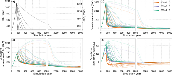
Figure 1. Timeseries of the (a) applied CO2 forcing (left y-axis and grid lines) and resulting change in atmospheric carbon inventory (right y-axis), (b) total cumulative emissions, change in the (c) cumulative atmosphere-ocean carbon flux, and (d) cumulative atmosphere-land biosphere carbon flux. Colors indicate equilibrium climate sensitivities. The lighter the color, the lower the CDR rate. Shown is the difference to a corresponding control run.
Download figure:
Standard image High-resolution imageCumulative carbon emissions to the atmosphere (figure 1(b)) are calculated for any period by summing the prescribed changes in the atmospheric carbon inventory (conversion: 2.12 GtC ppm−1; figure 1(a), left axis) and the simulated changes in the cumulative atmosphere-ocean (figure 1(c)) and atmosphere-land biosphere (figure 1(d)) carbon fluxes.
3. Results
3.1. Carbon cycle responses
We first illustrate changes in the global carbon cycle budget (figure 1). Diagnosed cumulative emissions depend on ECS and the CDR rate. Generally, cumulative emissions are higher for low ECS than for high ECS and are in the range of 2 640 (ECS = 5 °C) to 2 885 GtC (ECS = 2 °C) in year 140 (figure 1(b)) when atmospheric CO2 peaks at 4 × preindustrial (figure 1(a)). Cumulative emissions start to decline for all ECS with the onset of carbon dioxide removal (CDR), except for very slow CDR rates.
Anthropogenic carbon is redistributed in the Earth system (figure 1). The carbon uptake or release by the ocean depends on the difference in CO2 partial pressure in the ocean and atmosphere,  pCO2 = pCO
 pCO
pCO (McKinley et al
2020) and is governed by surface-to-deep mixing.. The ocean is the dominant net carbon sink. At peak CO2 (year 140), 1 805 GtC have entered the atmosphere, 645 GtC the ocean, and 355 GtC the land biosphere for an ECS of 3 °C. The ocean continues to take up CO2 for a few more centuries under slow CDR rates, as equilibrium is not yet reached due to the slow ocean overturning. For a CDR rate of 0.1 %yr−1, for example, the oceanic sink peaks at 1 260 GtC (ECS = 5 °C) to 1 420 GtC (ECS = 2 °C) around simulation year 780.
(McKinley et al
2020) and is governed by surface-to-deep mixing.. The ocean is the dominant net carbon sink. At peak CO2 (year 140), 1 805 GtC have entered the atmosphere, 645 GtC the ocean, and 355 GtC the land biosphere for an ECS of 3 °C. The ocean continues to take up CO2 for a few more centuries under slow CDR rates, as equilibrium is not yet reached due to the slow ocean overturning. For a CDR rate of 0.1 %yr−1, for example, the oceanic sink peaks at 1 260 GtC (ECS = 5 °C) to 1 420 GtC (ECS = 2 °C) around simulation year 780.
The ocean turns from a sink to a source during CDR because CO2 is removed from the atmosphere and  pCO2 becomes positive. In turn, the cumulative atmosphere-ocean C flux begins to decrease. The timing and magnitude of the sign change depends primarily on the CDR rate. The faster the CDR, the earlier the ocean turns from a sink into a source. In all cases, the ocean releases carbon to the atmosphere for centuries to millennia after CO2 is stabilized at preindustrial concentration (c.f. figures 1(a) and (c)). The cumulative atmosphere-ocean C flux varies slightly among ECS; a smaller oceanic sink for higher ECS follows from lower CO2 solubility under higher temperatures and larger reductions in overturning (c.f. figures 1(c) and 2(a), (c)).

Figure 2. Timeseries of the anomalies (Δ) in the (a) global mean surface air temperature (SAT), (b) total ocean heat content (OHC), (c) maximum strength of the Atlantic meridional overturning circulation (AMOC), and (d) remaining fraction of global sea-ice area. Colors as in figure 1.
Download figure:
Standard image High-resolution imageThe cumulative atmosphere-land biosphere flux increases and declines largely in concert with CO2 and SAT (figure 1(d)). CO2 fertilization of plants stimulates carbon uptake under higher atmospheric CO2 and respiration is enhanced under higher temperatures. The land biosphere sequesters about 250 GtC less in soils and litter (∼170 GtC), and vegetation (∼80 GtC) under high than low warming, mainly due to enhanced temperature-driven respiration (figure 1(d)). The cumulative atmosphere-land biosphere flux declines with CO2 to approach zero for low and intermediate ECS. Under high ECS, the cumulative flux becomes temporarily negative. Thus, the land biosphere stores less carbon than at preindustrial. This highlights the risk that the land biosphere may not only loose excess 'anthropogenic' carbon, but even some of its 'natural' carbon inventory. The latter represents an irreversibility with potential long-term consequences for ecosystems and ecosystem services.
On millennial timescales, CaCO3 compensation adds up to 200 GtC to the ocean. For most scenarios and by the end of the simulations, the cumulative contribution from sedimentation-weathering imbalances in the CaCO3 cycle ranges between an addition of 40 GtC to a removal of 20 GtC, and no new equilibrium is reached. CaCO3 compensation changes alkalinity twice as much as carbon, leading to changes in the carbon uptake capacity of the ocean, explaining the long-term perturbation in the cumulative atmosphere-ocean C flux (figure 1(c)). Imbalances in the sedimentation-weathering cycle of particulate organic carbon (POC) are small and mainly result from changes in POC preservation under lower O2.
3.2. Physical responses
 SAT rises in response to higher CO2 forcing (figure 2(a)), and at maximum cumulative emissions amounts to 2.7 °C, 3.7 °C, and 5.4 °C for ECSs of 2 °C, 3 °C, and 5 °C, respectively. The spatial warming pattern at maximum emissions resembles the global warming pattern for RCP 8.5 scenarios (IPCC 2013), with largest warming in high latitudes and over continents. Continued warming after maximum emissions scales with the subsequent removal rate and ECS. After returning to initial CO2 concentrations, it takes centuries to millennia before SAT returns to its preindustrial value. The slower the CDR and the higher the ECS, the longer SAT stays elevated (figure 2(a)). Slow CDR scenarios and a high ECS yields
  SAT of up to 1 °C at the end of the simulation, while for ECS = 2 °C remaining
  SAT is below 0.1 °C.
 OHC is, similar to
  SAT, largest for high ECS and slow CDR (figure 2(b)) and keeps increasing after maximum emissions. The surface ocean heat content equilibrates rather fast with the atmospheric temperature perturbation, while equilibration of the deep ocean is slow, with circulation as the rate limiting step. Thus, the slower the CDR, the longer the radiative imbalance lasts and the more of the perturbation will be transported to the deep ocean. Total OHC increases as long as the net downward heat flux at the top of the atmosphere is positive, resulting in an increase of
  OHC by a factor
  2–3 after maximum CO2, depending on CDR (see e.g. light colors in figure 2(b)).
 AMOC is reduced by 4.8–8.8 Sv at maximum CO2 forcing, depending on ECS and thus the corresponding temperature perturbation (figures 2(a) and (c)). AMOC starts to recover with declining forcing and overshoots to higher than initial values in all scenarios. The maximum overshoot is reached when CO2 concentrations are back to initial. By the end of the simulations, AMOC states differ. Similar to SAT, slow CDR scenarios with an ECS of 5 °C show strongest deviations in AMOC strength at simulation year 5 000 and across the ensemble of runs. From the available simulations it is not clear if and when the AMOC would return to its initial strength.
Sea-ice reacts fast to changes in SAT and is substantially reduced in both hemispheres (figure 2(d)). The reduction is larger for higher ECS. Sea-ice recovers over most of the simulations. For ECS = 2 °C, however, sea-ice area seems to stabilize at ∼95% of its initial cover. The slow recovery and partial reversion into a new reduction of sea-ice area during and after CDR (see e.g. orange lines around year 600 in figure 2(d)) is driven by Southern Hemisphere (SH) sea-ice changes. Generally, the reduction in the SH is larger than in the Northern Hemisphere (NH) and longer lasting.
3.3. Hysteresis
We quantify hysteresis as the difference in a variable between the up-path with increasing cumulative emissions and the down-path with decreasing cumulative emissions at 1000 GtC of cumulative carbon emissions. We thus consider large overshoot scenarios of up to about 2000 GtC (figure 1(b)).
We first examine differences in SAT between the up-path (dashed lines) and down-path (solid lines; figure 3(a)). Generally, the higher the ECS, the larger the hysteresis (see bars at the right of figure 3(a)). Non-linearities in SAT in the cumulative emission space do not scale linearly with ECS. For an ECS of 2 °C, hysteresis is small and largely negative. With ECS = 3 °C, SAT is in the mean 0.1 °C higher for the down- than up-path, while for ECS = 5 °C this difference increases to 1.5 °C. This means that at cumulative emissions of 1000 GtC and an ECS of 2 °C temperatures are mostly lower on the down-path compared to the up-path, while for ECS of 3 and 5 °C they are higher.
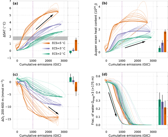
Figure 3. Hysteresis for (a)  SAT, (b)
  upper ocean (0–700 (m) heat content, (c)
  O2 in the thermocline (200 m–600 m), and (d) fraction of water with aragonite saturation state
  3. Bar plots show the mean and ±1 standard deviation of the hysteresis at 1 000 GtC cumulative emissions (vertical dashed purple line) across all CDR rates for each ECS (colors). Grey shading in (a) shows the range of 1.5–2 °C warming. The upward CO2 path is indicated by the arrows and dashed lines. It lasts 140 years, while the CO2 decline and stabilization period (solid lines) extends over 4860 years. Colors as in figure 1.
Download figure:
Standard image High-resolution imageUpper ocean (700 m) heat content (OHC700, figure 2(b)) shows similar hysteresis as SAT. With decreasing cumulative emissions, OHC700 first keeps increasing, until atmosphere and upper ocean are in equilibrium. For all three ECS, the mean hysteresis width is positive and ranges between 0.4 and 1.8 1024 J.
Changes in O2 result from changes in O2 consumption due to remineralization, from changes in O2 solubility, and to a lesser extent from changes in air-sea disequilibrium. Remineralization-driven changes in O2 correlate well with changes in ideal age (not shown): the weaker the ventilation and thus the older the water masses, the more oxygen is consumed by remineralization of organic matter. In many regions, ocean overturning circulation and ventilation is reducing under global warming causing O2 to decline. Higher temperatures at the surface lead to lower O2 solubility and lower surface concentrations which are then transported to the ocean interior. Reductions in thermocline O2 are larger for higher than lower ECS (figure 3(c)). The mean hysteresis width for an ECS of 5 °C is about –4 mmol m−3, while for ECS = 3 °C and ECS = 2 °C it is positive.
In contrast to SAT or O2, changes in  depend weakly on the ECS, but vary with the rate of CDR (figure 3(d)).
  decreases with increasing dissolved CO2. Therefore,
  follows the increase and decline in atmospheric CO2 without much delay in near surface waters and with delay in the deep ocean. At atmospheric CO2 of about 565 ppm and cumulative emissions close to 1 000 GtC, there are almost no waters left with
  3. The decrease in cumulative emissions is delayed relative to the decrease in atmospheric CO2, and
  starts to recover at much higher cumulative emissions during the down-path relative to the up-path. This hysteresis is particularly large for low CDR rates (figure 3(d)). Recovery of
  is generally faster for low ECS in the cumulative emissions space, resulting from larger contributions of changes in ocean and land carbon to the emission budget (see figure 1). CDR is potentially highly effective in mitigating near surface ocean acidification quickly, but deep ocean acidification is, as the perturbation in ocean carbon (figure 1(c)), long-lived.
3.4. Spatial patterns of hysteresis
Next, we focus on the spatial patterns of hysteresis in SAT and O2 and how they vary with ECS. We compare spatial anomalies for the CO2 down-path minus the up-path at cumulative emissions of 1 000 GtC and a CDR rate of 1 %yr−1 (figure 4). 1 000 GtC are reached in simulation year 67, 68, and 69 on the up-path, and in simulation year 257, 249, and 231 on the down-path for ECS of 2 °C, 3 °C, and 5 °C, respectively. We again consider large levels of overshoot above the baseline of 1 000 GtC.

Figure 4. Hysteresis in (a), (c), (e) SAT and (b), (d), (f) thermocline O2 (down-path minus up-path at cumulative emissions of 1 000 GtC). Results are for a decrease rate of 1 % yr−1 and for ECSs of (a), (b) 2 °C, (c), (d) 3 °C, and (e), (f) 5 °C.
Download figure:
Standard image High-resolution imageThe hysteresis of SAT is largely negative for an ECS of 2 °C and becomes positive for higher ECS (figures 3(a) and 4(a), (c) and (e)). A clear polar amplification is visible across all three ECSs. Highest positive temperature differences are located over Alaska and Eastern Siberia and in the Bering and Chukchi Seas, and in the Atlantic sector of the Southern Ocean. These regions show reduced sea-ice area and thus a lower albedo for the down-path compared to the up-path (see figure 2(d)).
Thermocline O2 shows spatially varying positive and negative hysteresis. Hysteresis of O2 is negative in the Arctic, the Atlantic south of the equator, and most of the Pacific. The Atlantic north of the equator and the northern Pacific show large positive hysteresis in thermocline O2 (figures 4(b), (d) and (f)). The pattern is generally comparable between different ECSs. In parts of the North Pacific and in the Southern Ocean, however, thermocline O2 shows positive hysteresis for ECSs of 2 °C and 3 °C, while for ECS = 5 °C the hysteresis is negative. The hysteresis patterns result from the interplay of consumption of O2 during remineralization, ventilation of water masses, and contributions from temperature anomalies to the solubility component of oxygen, O . Hysteresis in thermocline O
 is generally negative, except in the Southern Ocean for ECS of 2 and 3 °C with slightly positive values (not shown). The most negative O
 differences coincide with the O2 hysteresis minima in the Arctic and the Atlantic south of the equator.
The Indian Ocean, the tropical Western and Northeastern Pacific, the Atlantic north of the equator and the Atlantic sector of the Southern Ocean show minima in ideal age hysteresis (not shown), indicating higher ventilation of waters in the thermocline. Directly around Antarctica, water mass age increases for ECS = 5 °C. On top, export production exhibits most negative hysteresis in the North Atlantic in response to a weaker AMOC and thus reduced nutrient supply, and most positive hysteresis around Antarctica as a result of reduced sea-ice cover. Together, reduced water mass age and less export production lead to less oxygen consumption (i.e. Indian Ocean, Atlantic north of the equator, parts of the Pacific), while less ventilation and increased export production as seen around Antarctica yield lower O2 on the down-path than on the up-path for ECS of 2 °C and 3 °C (figures 4(b) and (d)). For ECS = 5 °C, and to a lesser extent ECS = 3 °C, negative hysteresis in O and positive hysteresis in ideal age around Antarctica lead to the sign change in O2 hysteresis there (figures 4(d) and (f)).
Finally, in the case of  , differences between the three ECS are small (figure 3(d)). Ωarag
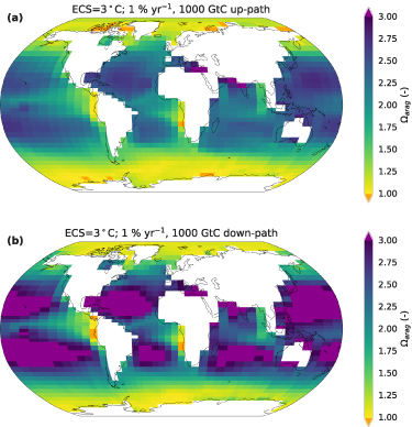
is generally lower during rising CO2 than during CDR for the same cumulative emissions (figures 3(d) and 5). The recovery is strongest in the sub-tropics, where
, differences between the three ECS are small (figure 3(d)). Ωarag
is generally lower during rising CO2 than during CDR for the same cumulative emissions (figures 3(d) and 5). The recovery is strongest in the sub-tropics, where  reaches values
  3 in most areas (figure 5(b)). The tropics show slightly higher
  values for CDR compared to emissions, while the high latitudes are similar for the two time slices (figure 5).
Figure 5. Mean aragonite saturation state ( ) of the uppermost 175 m (first four vertical layers in the model) for cumulative emissions of 1 000 GtC on the (a) up-path and (b) down-path, and an ECS of 3 °C and a CDR rate of 1 %yr−1.
Download figure:
Standard image High-resolution image
4. Discussion
Results from our experiments with different, highly idealized carbon dioxide removal (CDR) rates for three different equilibrium climate sensitivities (ECS) have several implications. The response in global mean surface air temperature (SAT) to positive cumulative carbon emissions is nearly linear and has been used to calculate the remaining carbon budget in order to reach certain climate targets (e.g. Matthews et al
2009, Steinacher et al
2013, IPCC 2013, Stocker 2013, Goodwin et al
2015, Rogelj et al
2019). Similarly, the proportionality between SAT (and many other variables) and atmospheric CO2 (e.g. Armour et al
2011, Boucher et al
2012, Li et al
2013) and cumulative emissions (e.g. Zickfeld et al
2016) has been investigated for idealized CDR. In the case of SAT, for example, a non-linear response during the up- and down-path of CO2 has been found, as in this study. With higher ECS, however, this non-linearity in the cumulative emissions space increases in the large overshoot scenarios considered here (figure 3(a)). The remaining carbon budget should, therefore, not be computed from the established relationship between positive cumulative carbon emissions and  SAT (Allen et al
2009, Stocker et al
2013b) for high overshoot scenarios with CDR. This non-linearity implies that in order to return to a certain temperature with the help of CDR requires the removal of more carbon than was emitted after passing the same temperature on the up-path (see also MacDougall 2013, MacDougall et al
2015).
SAT (Allen et al
2009, Stocker et al
2013b) for high overshoot scenarios with CDR. This non-linearity implies that in order to return to a certain temperature with the help of CDR requires the removal of more carbon than was emitted after passing the same temperature on the up-path (see also MacDougall 2013, MacDougall et al
2015).
Other physical and biogeochemical variables such as changes in ocean heat content, AMOC strength, or thermocline O2 show, as SAT, increasing hysteresis with higher ECS, while for the Ωarag saturation state hysteresis is smaller under high ECS. Potentially higher ECS of the Earth system than previously assessed (Forster et al 2020), underscores the urgency of emissions reduction to net zero (see also discussion below).
There are several limitations to our study. First, we use an Earth system model of intermediate complexity (EMIC). Besides the benefits, such as the possibility to cover a wide range of CDR rates for different ECSs and to run the model for several millennia, EMICs come with drawbacks. Many processes are implemented as simplified parameterizations, the atmosphere consists of an energy-moisture balance model with no atmospheric dynamics. For example, the cloud feedback is only indirectly parameterized in the Bern3D, with possible implications for the response to changes in radiative forcing (see e.g. Andrews et al 2015). Also, changes in continental ice-sheets are not simulated by the model but might well affect, for example, the response in AMOC. Nevertheless, the Bern3D-LPX model has been shown to perform well in comparison to observational data (e.g. Roth et al 2014) and comparable to other models in model intercomparison projects (Joos et al 2013, Eby et al 2013, MacDougall et al 2020), and has been used in several studies investigating the Earth system response to different emission scenarios (e.g. Steinacher et al 2013, Steinacher and Joos 2016, Pfister and Stocker 2016, Battaglia and Joos 2018).
Second, we apply highly idealized scenarios. Our maximum CO2 forcing corresponds to a 4 × CO2 scenario, comparable to a high emission scenario such as the Shared Socioeconomic Pathway (SSP) 5–8.5 (Riahi et al 2017). Future efforts might focus more on scenarios in line with the UNFCCC Paris Agreement's goal of holding global warming well below 2 °C. Previous studies show that the hysteresis in SAT varies with the amount of overshoot (Boucher et al 2012, Zickfeld et al 2016, Tokarska et al 2019). For small overshoots of the carbon budget of up to 300 GtC, SAT shows almost no hysteresis (Tokarska et al 2019), while it is larger for high overshoot scenarios (MacDougall et al 2015, Zickfeld et al 2016).
Third, concerning the chosen range of ECS, there is a large body of literature on estimates of the ECS of the Earth system. The last IPCC report concluded the ECS to lie within 1.5 to 4.5 °C with a probability of 66% (IPCC 2013). The review by Sherwood et al (2020) suggests for the effective climate sensitivity a 66% probability range of 2.6–3.9 °C, which remains within the bounds 2.3–4.5 °C under plausible robustness tests. This is consistent with earlier Bern3D observation-constrained estimates (2.0–4.2 °C; 68% range (Steinacher and Joos 2016)). The concept of equilibrium or effective climate sensitivity does not (or hardly) account for slowly evolving Earth System feedbacks (Heinze et al 2019), e.g. those associated with ice sheet albedo changes and many feedbacks involving biogeochemical cycles and GHGs. Here, we implicitly account for these additional feedbacks, beyond the carbon cycle-climate feedbacks explicitly modelled in Bern3D-LPX, by using an upper bound of 5 °C for ECS.
In summary, the response of the Earth system to positive and negative CO2 emissions differs. This hysteresis is sensitive to the choice of equilibrium climate sensitivity and carbon dioxide removal rate in the Bern3D-LPX model. Further, we investigate emission scenarios featuring a large level of overshoot above a chosen baseline of 1 000 GtC cumulative emissions. Generally speaking, our results suggest that no emissions is a better strategy than carbon dioxide removal, even if technologies existed to remove CO2 from the atmosphere and store it away safely and permanently. Negative emissions are considered in scenarios with a 1.5 °C warming target (IPCC 2018) as the required rate of emissions reduction seems unrealistically fast without allowing for an overshoot in temperature and subsequent CDR.
Acknowledgments
AJT acknowledges support from the Oeschger Centre for Climate Change Research.
TFS acknowledges funding from the Swiss National Science Founation (SNF 200020_172745) and the EU Commission (H2020 project TiPES, grant 820970). This is TiPES contribution #53. FJ acknowledges funding from Swiss National Science Foundation (SNF 200020_172476) and the from the European Union's Horizon 2020 research and innovation programme under grant agreement No 820989 (project COMFORT, Our common future ocean in the Earth system—quantifying coupled cycles of carbon, oxygen, and nutrients for determining and achieving safe operating spaces with respect to tipping points). The work reflects only the authors' view; the European Commission and their executive agency are not responsible for any use that may be made of the information the work contains.
Data Availability
The data that support the findings of this study are available upon reasonable request from the authors.