

Abstract
Remaining carbon budget specifies the cap on global cumulative CO2 emissions from the present-day onwards that would be in line with limiting global warming to a specific maximum level. In the context of the Paris Agreement, global warming is usually interpreted as the externally-forced response to anthropogenic activities and emissions, but it excludes the natural fluctuations of the climate system known as internal variability. A remaining carbon budget can be calculated from an estimate of the anthropogenic warming to date, and either (i) the ratio of CO2-induced warming to cumulative emissions, known as the Transient Climate Response to Emissions (TCRE), in addition to information on the temperature response to the future evolution of non-CO2 emissions; or (ii) climate model scenario simulations that reach a given temperature threshold. Here we quantify the impact of internal variability on the carbon budgets consistent with the Paris Agreement derived using either approach, and on the TCRE diagnosed from individual models. Our results show that internal variability contributes approximately ±0.09 °C to the overall uncertainty range of the human-induced warming to-date, leading to a spread in the remaining carbon budgets as large as ±50 PgC, when using approach (i). Differences in diagnosed TCRE due to internal variability in individual models can be as large as ±0.1 °C/1000 PgC (5%–95% range). Alternatively, spread in the remaining carbon budgets calculated from (ii) using future concentration-driven simulations of large ensembles of CMIP6 and CMIP5 models is estimated at ±30 PgC and ±40 PgC (5%–95% range). These results are important for model evaluation and imply that caution is needed when interpreting small remaining budgets in policy discussions. We do not question the validity of a carbon budget approach in determining mitigation requirements. However, due to intrinsic uncertainty arising from internal variability, it may only be possible to determine the exact year when a budget is exceeded in hindsight, highlighting the importance of a precautionary approach.
Export citation and abstract BibTeX RIS

Original content from this work may be used under the terms of the Creative Commons Attribution 4.0 license. Any further distribution of this work must maintain attribution to the author(s) and the title of the work, journal citation and DOI.
1. Introduction
Global warming is approximately proportional to the total amount of CO2 emitted [1, 2]. This ratio of CO2-induced warming to cumulative CO2 emissions during the period when emissions and atmospheric CO2 are increasing, is defined as the Transient Climate Response to cumulative CO2 Emissions (TCRE), and provides the basis for the concept of carbon budgets. A carbon budget is the total amount of CO2 that can be emitted while limiting global temperature change to below a particular threshold with a given probability (see Rogelj et al [3]. for a comprehensive comparison of the most recent carbon budget estimates for stringent temperature levels). The remaining carbon budget in a similar way refers to the amount of CO2 from the present day onwards that can still be emitted while limiting warming to below a particular threshold.
The IPCC Special Report on 1.5 degrees (SR1.5; Rogelj et al [4]) introduced a new framework for estimating remaining carbon budgets directly from TCRE, while integrating a separate quantification of the influence of non-CO2 scenario uncertainty, and other sources of uncertainties (i.e. Earth system response to non-CO2 forcing uncertainty, TCRE distribution uncertainty (normal vs. log-normal), historical temperature uncertainty, recent emissions uncertainty; see SR1.5 [4] table 2.2 therein). Here we refer to this framework as approach (i) of calculating remaining carbon budgets. For a comprehensive description of this framework see Rogelj et al [3, 4]; and a short summary provided in Methods section 2.3 below. Approach (i) is a step-change in the methodology of estimating remaining carbon budgets, as previous approaches -here referred to as approach (ii)—e.g. in IPCC AR5 –Collins et al [5]. and studies following it, were primarily based on estimating remaining budgets from a limited number of scenarios (e.g. Representative Concentration Pathways; RCP; Stocker et al [2]) that only indirectly reflect on an estimate of TCRE. A major limitation of approach (ii) is that the few RCP scenarios are subject to specific assumptions about future non-CO2 emissions, and may not be representative of the entire spectrum of scenarios that lead to stabilizing global mean warming at 1.5 °C or 2.0 °C, where CO2 emissions reach a net-zero level once the warming target is reached. In this paper, we examine the contribution of internal variability in the anthropogenic warming estimate, and quantify the impact of internal variability on the remaining carbon budgets calculated using either approach (i) or (ii), as well as the role of internal climate variability on the TCRE diagnosed from individual models.
The unforced internal variability in the climate system arises from sources such as the El Niño‐Southern Oscillation changes [6]. This paper studies the role of the unforced natural variability in future projections. The temperature limits of the Paris Agreement (1.5 °C and 'well below' 2.0 °C) are usually interpreted as levels of anthropogenic warming [7, 8], that by definition, are not subject to internal variability or 'noise' in the climate system. However, such a noise-free anthropogenic forced signal cannot be directly observed, and it is challenging to estimate it from a single realisation of the observational records. Some metrics that intend to estimate the anthropogenic contribution to the observed warming, such as the anthropogenic warming index [9] (AWI), are also uncertain, in part, due to internal variability. Furthermore, different observational products need to be reconciled [10]. SR1.5 (Rogelj et al [4]) assessed this uncertainty in historical warming due to differences in the observational products as ±0.12 °C (1σ range; SR1.5 SPM statement A1.1).
TCRE and remaining carbon budgets in approach (i) are determined by the temperature response to the total amount of CO2 emitted in the atmosphere (see Methods section 2.3). In a climate model environment, TCRE can, in principle, be estimated from the averaged forced response of a large ensemble, in which the internal climate variability is strongly reduced by ensemble averaging. However, most climate models report only one or very few simulations, each with their specific realisation of internal climate variability. Furthermore, a large ensemble approach remains limited to the model world, where multiple realisations of the climate projections are possible.
Another way of estimating remaining budgets is approach (ii), where the budgets are calculated directly from climate model simulations (e.g. Threshold Exceedance Budgets; see Methods section 2.3 and Rogelj et al [11]). This method assesses when either net warming or anthropogenic warming exceeds a temperature threshold. However, warming in comprehensive climate models is also influenced by internal variability. There is currently no single best approach to estimate the anthropogenic component of temperature change in a given year. For example, IPCC AR5 (Collins et al [5]) used a decadal running mean of individual model simulations [5, 11] to estimate carbon budgets consistent with 1.5 °C or 2.0 °C.
Here we quantify how internal variability contributes to uncertainty in TCRE and anthropogenic warming estimates, thereby limiting the accuracy with which remaining carbon budgets can be estimated (using either approach). We compare different methodological choices that smooth temperature time series in order to estimate the forced response (i.e. free from internal variability). Together with large ensemble averaging, we estimate the uncertainty in TCRE due to internal variability, and potential spread in the remaining carbon budgets if the budgets were estimated using approach (i), i.e. the SR.1.5 method. We also quantify the spread in remaining carbon budgets calculated directly from large ensembles of SSP and RCP scenarios (i.e. approach (ii), Meinshausen et al [12, 13]), noting, however, that such approach is no longer recommended for estimating the remaining carbon budget. A better understanding and quantification of the uncertainty due to internal variability is essential for risk assessments and other climate services or adaptation strategies that make use of climate model output.
2. Methods
2.1. Sinks and sources of atmospheric CO2
Anthropogenic CO2 emissions increase the atmospheric CO2 burden, while land and ocean currently take up about half of the emitted anthropogenic CO2 [14, 15]. Since the total amount of carbon in the atmosphere-ocean-land system is conserved, with the exception of input from fossil fuel emissions, total cumulative fossil fuel CO2 emissions ( ) may be partitioned into the change in atmospheric carbon burden (
 ), carbon uptake by the land (
 ) and carbon uptake by the ocean (
 ), expressed by equation (1).

The net ocean carbon uptake is predominantly driven by the increase in atmospheric CO2 concentration. The net carbon uptake over land is the result of three primary competing processes: (1) the natural carbon cycling through the vegetation-litter-soil continuum, which responds to rising atmospheric CO2 (through the CO2 fertilization effect); (2) the effect of associated change in physical climate (e.g. increase in temperature, change in precipitation patterns, etc.); and (3) the carbon loss over land due to land-use and land-cover changes (particularly relevant for historical and future emission scenarios). The change in carbon pool over land can therefore be expressed as the sum of changes due to the natural land carbon pools' response to changes in atmospheric CO2 and climate ( ), and due to anthropogenic land-use change (LUC) processes, where
  represents the cumulative LUC emissions and includes the effects of the reduced natural land carbon sink due to LUC. The carbon uptake by land (
 ) can thus be expressed as:
  (following Arora et al [16, 17]). Rearranging the terms of the total cumulative emissions (equation (1)) yields:

The term  is the terrestrial sink. Most Earth System Models (ESMs) simulate processes related to LUC interactively, and it is not possible to diagnose
  without another simulation that does not include anthropogenic LUC.
  can typically be diagnosed by differencing
  from simulations with and without LUC [18].
In the absence of such simulations with and without LUC for the models considered here, we use an estimate of the values of CO2 emissions from LUC,  , for the historical period and for the respective future SSP and RCP scenarios using estimates from [19], as was done in earlier studies [5, 20, 21]. We acknowledge that this estimate of LUC emissions differs from the actual LUC emissions that each model generates. However, since the primary purpose of this study is to quantify the role of internal variability on carbon budgets rather than to provide an exact estimate of the remaining carbon budget, the use of specified
  is not expected to influence our conclusions. Note that LUC emissions are not relevant for estimating TCRE in CO2-only simulations, as explained in section 2.2.
2.2. Transient climate response to cumulative CO2 emissions
The relationship between CO2-induced warming and cumulative CO2 emissions has shown to be approximately linear for up to 2000 PgC emitted [1, 5, 22–24] and beyond [25, 26], and largely independent of CO2 emission pathway for a wide range of CO2 -only pathways [27, 28]. The linearity of this relationship breaks down only for very low or very high emission rates [29].
The TCRE [1, 5] is expressed as a ratio of CO2-induced global mean warming ( ) to total cumulative CO2 emissions (
 ), expressed by equation (4). Cumulative CO2 emissions are inferred as the sum of all right-hand-side terms in equation (2), since the simulations considered here are driven by CO2-concentrations (as opposed to driven by CO2 emissions). We calculated
  and
and  as the time-integrated atmosphere-land and atmosphere-ocean carbon fluxes ('nbp' and 'fgco2' CMIP variable names). We use the global mean surface air temperature with full global coverage (GSAT), that is directly diagnosed from the ESM output ('tas' CMIP variable).
TCRE (equation (4)) was originally defined [1] using 1pctCO2 concentration-driven simulations in which atmospheric CO2 increases at a constant rate of 1% per year. Concentrations of all other non-CO2 climate forcings and land cover in the 1pctCO2 simulation stay at their pre-industrial level and therefore, emissions from LUC are zero ( ; section 2.1).
In addition to 1pctCO2 simulations, we also consider all-forcing simulations, which include both CO2 and non-CO2 forcing agents, in addition to natural forcing (solar and volcanic), and anthropogenic LUC (equation (3)). Warming as a function of cumulative emissions computed from such all-forcing simulations is referred to as the effective TCRE [30], and the presence of non-CO2 forcing makes it non-linear and dependent on the pathway of non-CO2 emissions [21, 31, 32]. Furthermore, emissions from LUC differ among such scenarios and are difficult to diagnose from the standard model output (see section 2.1). As noted in section 2.3, it is no longer recommended [3] to estimate remaining carbon budgets from the effective TCRE in RCP and SSP scenarios.
2.3. Remaining carbon budgets
A remaining carbon budget can be calculated from an estimate of the anthropogenic warming to date (discussed in the next section 2.4), and either (i) the ratio of CO2-induced warming to cumulative emissions, known as the TCRE, in addition to information on the temperature response to the future evolution of non-CO2 emissions; or (ii) climate model scenario simulations that reach a given temperature threshold.
2.3.1. Approach (i): SR 1.5 framework for estimating remaining carbon budgets
The SR1.5 (Rogelj et al [4] and Rogelj et al [3]) introduced a new framework for estimating remaining carbon budgets, that makes use of TCRE to infer the CO2 carbon budget, and allows for more specific treatment and assessment of uncertainty due to future non-CO2 scenario variation under a broad spectrum of scenarios. Additional sources of uncertainty, such as unrepresented Earth System feedbacks, are accounted for separately (see SR1.5 table 2.2 and Rogelj et al [3]. for detail). This new approach leads to more explicit quantification of different sources of uncertainty in the remaining carbon budgets, while also allowing for calculating remaining carbon budgets for a specific mix of non-CO2 forcings consistent emission pathways that lead to net-zero CO2 emissions. Using this approach minimizes the uncertainty in the cumulative CO2 emissions, which, may differ among ESMs in the historical period (see Rogelj et al [3] and Tokarska et al [33] for further discussion of the advancements in the recent methodologies to obtain more accurate remaining carbon budget estimates). It is currently the recommended method of estimating remaining carbon budgets, rather than using the previous approach (ii) described below.
2.3.2. Approach (ii): threshold exceedance budgets (IPCC AR5 and studies following it)
Estimating remaining carbon budgets directly from the all-forcing simulations (such as SSP and RCP scenarios) was an approach used in AR5 (Stocker et al [2, 5]) and studies following it. Such carbon budgets are referred to as 'threshold exceedance carbon budgets' as they are calculated from scenarios in which emissions, by design, continue to increase, and do not entail a smooth transition to a net-zero emission level by the time the budget is reached (i.e. by design, the temperature target could be exceeded in the year following the budget cap). However, recently, several shortcomings have been identified in that approach [3], including limits to the usefulness of such threshold exceedance budgets. These SSP and RCP scenarios do not represent emission pathways that lead to net-zero emissions, and their non-CO2 forcing is hence representative of a continued-warming future instead of a future in which global warming is halted. Furthermore, the limited set of SSP and RCP-based scenarios include only a few possible future non-CO2 forcing evolutions, which may not be representative of the entire spectrum of possible future non-CO2 combinations that are compatible with stabilizing warming at levels consistent with the Paris Agreement (e.g. compared to the scenarios in the SR1.5 database [34, 35]). Thus, we do not provide remaining budget estimates based on CMIP6 SSP and CMIP5 RCP simulations. We only report the spread in the remaining budgets that arise from using a single ensemble member (or limited size ensemble), when calculating the remaining budgets directly from those scenarios, for illustrative purposes.
2.4. Anthropogenic warming estimate
Paris Agreement temperature limits may be interpreted as levels of anthropogenic warming [5, 6], that by definition, are not subject to internal variability. To estimate the anthropogenic contribution to the observed warming, the [8] AWI can be used, by regressing out the natural influence. However, the AWI estimate is affected by internal variability in the observations. The uncertainty range due to internal in AWI can be estimated based on pre-industrial control variability, which is based on pre-industrial control simulations of CMIP5 models [8, 30]. Either method of calculating the remaining carbon budgets from the present-level day warming (either the SR1.5 approach or the previously used threshold exceedance approach) requires an estimate of the anthropogenic warming to-date, in order to know how much warming is left until the 1.5 C or 2.0 °C target, for example. Remaining carbon budgets are more accurate than the total carbon budgets, as using the present-day baseline reduces the overall uncertainty in carbon budget estimates [33].
2.5. Model simulations
We use simulations from climate models participating in the CMIP5 and CMIP6 intercomparisons [36, 37] that had ensemble sizes of at least five members available in all-forcing simulations, and single ensemble members from 1pctCO2 simulations (listed in Supplementary table S1 (available online at stacks.iop.org/ERL/15/104064/mmedia)). The three models with the largest ensemble sizes are: the Canadian Earth System Model (CanESM2) with a 50-member ensemble [16, 38]; CanESM5 with a 50-member ensemble [39], and the MPI-ESM-GE grand ensemble of 100 members [40] (note that only 32 members of MPI-ESM-GE had carbon cycle output available in 1pctCO2 simulations used to calculate TCRE). In each model's ensemble, the differences among simulations are only due to internal variability of the climate system. Such variations can be simulated by perturbing a random seed within a stochastic component of the cloud parametrisation (in the case of CanESM2) [38], and/or by choosing a different initialization year from the pre-industrial control run from which a member of the historical simulation is initialized (in the case of MPI-ESM-GE) [40]. Each model simulation was driven with prescribed atmospheric CO2 concentration according to the historical forcing followed by the specified-concentration RCP 8.5 scenario [12] (in the case of CMIP5 models), or SSP 5–8.5 and SSP 2–4.5 scenarios [13] (in the case of CMIP6 models; Supplementary tables S1 and S2). These simulations include natural and anthropogenic forcing from CO2 and non-CO2 forcers [19]. We also use the 1pctCO2 simulations from models which contributed to CMIP6. These 1pctCO2 simulations were used to calculate TCRE values for the following models: CanESM5, CESM2, CNRM-ESM2-1, IPSL-CM6A-LR, MPI-ESM1-2-LR, NorESM2-LM, UKESM1-0-LL, ACCESS-ESM1-5, CESM2-WACCM, MIROC-ES2L (see Supplementary Material for a list of all models used for each type of simulation, and their respective ensemble sizes).
3. Results
3.1. Effects of internal variability on TCRE
Internal variability in the climate system can be quantified as uncertainty across the individual ensemble members in a large ensemble of simulations from each model, because each ensemble member is subject to identical forced radiative forcing (see Methods section 2.5). An estimate of the forced response (with internal variability removed) can be obtained by taking a mean of individual ensemble members of the same model. However, most models only provide one ensemble member in 1pctCO2 simulations, which is subject to internal variability. Some studies [41, 42] suggest that fitting a fourth-order polynomial to annual temperature time-series results in a reasonably good approximation of the forced response. Here we compare how different smoothing methods applied to the temperature response in 1pctCO2 simulations affect the resulting TCRE estimates.
The TCRE estimate obtained by fitting a fourth-order polynomial to individual ensemble members of the same model results in nearly the same value as taking the 32-member ensemble mean annual mean temperature in MPI-ESM-GE (figures 1(a) and (b)) and similar results are obtained for the 10-member ensemble of CNRM-ESM 2.1 (figures 1(c) and (d)). However, in both models, the likely range (17%–83%) and 5%–95% range is much narrower when the smoothing is applied, compared with the annual time-series (figures 1(b) and (d), first yellow bar compared with the last purple bar). The remaining uncertainty in TCRE calculated using a fourth-order polynomial results from variability on longer, multi-decadal time-scales that is not accounted for by the polynomial.
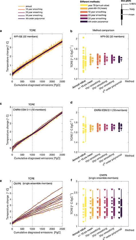
Figure 1. Comparison of uncertainty in TCRE due to internal variability, using different smoothing methods. (a,c) Temperature as a function of diagnosed cumulative CO2 emissions in MPI-ESM grand ensemble (32 members)[40] and CNRM-ESM2-1 (10 members) [43] in 1pctCO2 simulation; (b,d) TCRE range in each model using different smoothing methods, as labelled (5%–95%, likely 17%–83%, and mean value); (e) as in (a,b) but for CMIP6 models (one ensemble member per model) in 1pctCO2 simulation. (f) Resulting multi-model TCRE distribution calculated using different smoothing methods, as labelled.
Download figure:
Standard image High-resolution imageThe uncertainty in TCRE due to internal variability in individual models can be as large as ±0.1 °C/1000 PgC (5%–95% range) when temporal smoothing is applied in 1pctCO2 simulations in a single model (e.g. MPI-ESM-GE; figure 1(a) and (b), or CNRM-ESM2-1 in figure 1(c) and (d); see Supplementary table S2 for details). We note that a similarly narrow TCRE range can also be obtained by estimating TCRE as the 20-yr mean, centered on the year when 1000 PgC is emitted, which is the recommended way of obtaining the TCRE estimate [24]. The method of calculating TCRE does not influence the overall TCRE distribution in CMIP6 models appreciably, as model uncertainty dominates over the uncertainty due to internal variability and the method to calculate TCRE (figure 1(e)).
In principle, TCRE as a property of climate models based on the 1pctCO2 simulations, and the value of TCRE should be determined by the externally forced model response (free from the unforced internal variability). In practice, there are currently limitations to estimating TCRE without the influence of unforced internal variability as illustrated here, because often only one ensemble member is available per model in 1pctCO2 simulations. For similar analysis regarding the Transient Climate Response (TCR) estimates (i.e. warming in the year 70 of 1pctCO2 simulations) see Supplementary Material.
3.2. Contributions from internal variability to the remaining carbon budgets uncertainty
In this section, we investigate the influence of internal variability on remaining carbon budgets using the threshold exceedance approach (i) (Methods section 2.3). Despite smoothing to reduce the uncertainty, we still find a significant contribution to overall uncertainty from internal variability, especially for 1.5 °C budgets. The uncertainty in warming due to internal variability as a function of cumulative emissions (figure 1) implies that even within the same model and under the same scenario, the remaining carbon budget for a given level of warming (such as 1.5 °C) is not a single number, but rather a range of numbers, even after strong smoothing is applied to isolate the forced response. This remaining uncertainty in each model response arises due to internal variability in the climate system that acts on various time scales from multiple decades to multiple centuries, and is thus still present even once the inter-annual to decadal variability is removed. This uncertainty can be reduced but not eliminated entirely given current observational and model capacities. We quantify this uncertainty in the remaining carbon budgets in figure 2.
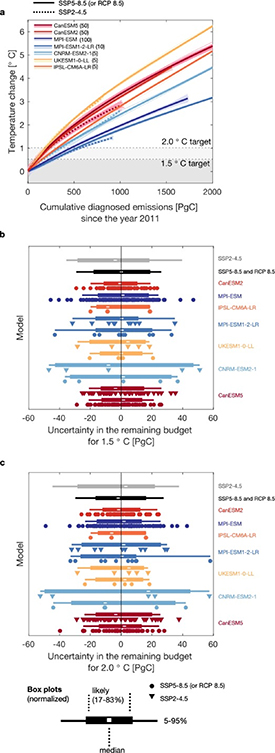
Figure 2. Effective TCRE and normalized uncertainty due to internal variability in remaining carbon budgets until 1.5 °C and 2.0 °C warming is reached. (a) Temperature as a function of cumulative CO2 emissions based on SSP 5–8.5 scenario (and RCP 8.5 for CanESM2 and MPI-ESM-GE) and SSP 2–4.5 scenarios, defined here as the forced response estimates by fitting fourth-order polynomials to individual ensemble members; (b) uncertainty in the remaining carbon budgets for 1.5 °C; (c) uncertainty in the remaining carbon budgets for 2.0 °C.
Download figure:
Standard image High-resolution imageHere, for illustration of the effect of internal variably in all-forcing scenarios, we calculate remaining carbon budgets for 1.5 °C and 2.0 °C, with respect to the 2006–2015 baseline, directly from the effective TCRE curve in SSP2-4.5, SSP5-8.5 and RCP 8.5 scenarios (figure 2), and reflect the amount of cumulative CO2 emissions in the year prior to which a given temperature target is exceeded (i.e. 'exceedance budgets' [11]). As noted in Methods section 2.3, this approach of calculating remaining carbon budgets is no longer recommended, as such threshold exceedance budgets calculated directly from ESM output under RCP and SSP scenarios are subject to assumptions on the particular mix of CO2 and non-CO2 forcings that have limited application for mitigation pathways in line with keeping warming to 1.5 °C or 2 °C. Recently, other methods (using TCRE values directly and estimates of future warming from non-CO2 forcing contributions) have been suggested to circumvent this issue (See Methods section 2.3 and Rogelj et al [3]).
The focus of our study is to analyse the uncertainty in the remaining carbon budgets due to internal variability, rather than their nominal values, and carbon budgets calculated directly from ESM output provide such an opportunity. Note that historical and future emission scenarios (such as SSPs and RCPs) are subject to anthropogenic and natural forcing (solar forcing and volcanic forcing), in addition to the unforced climate variability. We make the assumption that the ensemble mean of the simulations in a large ensemble including both anthropogenic and natural forcing is an estimate of the anthropogenic response (i.e. the natural response is assumed to be zero). While the natural forcing response is probably relatively small in both cases, it will not be exactly zero. This may affect the threshold exceedance carbon budgets, but not the carbon budgets calculated from TCRE directly (as TCRE is obtained from 1pctCO2 simulations; Methods section 2.2).
Internal variability affects the remaining carbon budgets for both the 1.5 °C and 2.0 °C limits by about ±30 PgC and ±40 PgC (5%–95% range for both sets of scenarios considered here; Supplementary table S3; figures 2(b) and (c)) even after estimating the forced temperature response by fitting fourth-order polynomials. Generally, differences among models contribute much more to the overall uncertainty than the differences due to internal variability. The influence of inter-model uncertainty can be minimized by adjusting the baseline period to the most recent period and calculating remaining budgets only from that point onwards and until a given temperature limit is reached [33]. In turn, the uncertainty due to internal variability is approximately constant and not affected by this change of baseline (since uncertainty in TCRE and remaining carbon budgets is dominated by the temperature component, and internal variability in temperature does not change much at different forcing levels [42]).
In figure 3 we illustrate relative contributions of internal variability and model uncertainty, for the models considered here, following Hawkins and Sutton [41, 42] approach of visualizing contributions of different uncertainty types. The relative contribution from internal variability is important and may exceed the model uncertainty on very short time-scales (as it is constant, irrespective of the baseline), but on longer time-scales, the inter-model spread dominates. Since the remaining carbon budget for 1.5 °C is close to the origin of the effective TCRE curve, with the 2006–2015 baseline (figure 2(a)), it is subject to relatively large uncertainty due to internal variability (figure 3(c)), as model uncertainty is assumed to be zero at the origin (by design due to the choice of a recent baseline). This relative contribution of internal variability to overall uncertainty diminishes for a 2.0 °C carbon budget (figure 3(d)), where model uncertainty starts to emerge and dominate.

Figure 3. Illustration of relative contributions to the total uncertainty in the temperature response to cumulative CO2 emissions and remaining carbon budgets (following the threshold exceedance budgets definition), separated into contributions due to model uncertainty and internal variability in the temperature response. (a) temperature as a function of cumulative CO2 emissions in SSP5-8.5 and RCP 8.5 scenario (effective TCRE), indicating contributions from model uncertainty and internal variability; (b) fractional contribution to total uncertainty as a function of cumulative CO2 emissions from 2011 onwards; panels (c) and (d) show zoomed-in portions of panel (b) until the 1.5 °C and 2.0 °C target is reached (where the point of reaching the target is based on a multi-model mean remaining carbon budget, as shown in panel (a)).
Download figure:
Standard image High-resolution imageWe note that figure 3 is for illustrative purposes only because only models for which large or medium-sized ensembles were considered. We also do not consider scenario uncertainty here, as for the time period and lead time considered there is no substantial difference in the effective TCRE between SSP5-8.5 and SSP2-4.5 (for the models considered here; figure 3(a)), and between RCP 8.5 and RCP 4.5 (Tokarska and Gillett [20]). However, the SSP and RCP scenarios represent only a small portion of all available scenarios, and for 1.5 °C and 2.0 °C targets, there are numerous combinations of non-CO2 and CO2 forcings to reach those targets. Therefore, ambitious mitigation targets (such as the Paris Agreement) are subject to large scenario uncertainty that would need to be explored beyond the RCP and SSP scenarios (for example, using climate model emulators and the SR1.5 scenario database [34, 35]). Such analysis is beyond the scope of this study that focuses primarily on the role of internal variability on TCRE and remaining carbon budgets, rather than an assessment of the overall uncertainty.
3.3. Challenges in estimating the anthropogenic warming (free from internal variability)
Estimating the remaining budget using either method -the SR1.5 approach (i) or the remaining threshold exceedance budgets approach (ii) based on AR5 requires a precise estimate of the present-day anthropogenic warming or mean warming at the time of the baseline period. The [9] AWI, is a method of assessing anthropogenic global mean warming for meeting the Paris Agreement target [3, 4] (Methods section 2.4). We qualitatively compare the uncertainty due to internal variability in AWI with the spread of the large ensemble (note that the definition of internal variability is not exactly the same between the two estimates, and AWI has the natural-only variability from solar and volcanic forcing influence removed [9]). Following Haustein et al [9], figure 4 shows the AWI calculated on a single ensemble member from the MPI-ESM-GE (black), which is treated as pseudo-observations. The resulting AWI and its overall uncertainty range is shown in orange, while the MPI-ESM-GE grand ensemble mean of 100 simulations is shown in dark blue. The spread due to internal variability in AWI (red shaded area) is similar to the spread of the 100 members of MPI-ESM-GE large ensemble (light blue lines), where individual ensemble members were smoothed using the fourth-order polynomial fits. The magnitude of the uncertainty due to internal variability (at 'present-day', i.e. by the end of these time-series, figure 4(b)) in both these methods is similar (though these uncertainty ranges are not a like-for-like comparison, as discussed above). Generally, the large ensembles approach estimate provides a reasonable way of characterising internal variability in a particular model. The uncertainty in AWI due to internal variability in the year 2019 is estimated at ±0.09 °C (figure 4 red shaded area; 5%–95% range), which corresponds to a contribution to uncertainty in remaining carbon budgets of about ±50 PgC (using a median estimate of TCRE of 1.65 °C/1000 PgC as in SR1.5 Rogelj et al [4]).

Figure 4. Comparison of uncertainty due to internal variability in estimates of anthropogenic warming, relative to 1850–1900 baseline. Uncertainty due to internal variability in the AWI index (based on Haustein et al [9].; run on a single ensemble member from the MPI model treated as 'pseudo observations'), and in the large ensemble spread of MPI-ESM-GE (100 member ensemble, using fourth-order polynomial smoothing), as labelled. Panel (b) shows a zoomed-in version of panel (a), more relevant for calculating the remaining carbon budgets using a recent baseline (e.g. 2006–2015).
Download figure:
Standard image High-resolution image
4. Discussion and conclusions
Temperature targets established under the Paris Agreement are interpreted in the context of anthropogenic climate change [7, 8]. To evaluate how the world is tracking with respect to such targets, and to derive the remaining carbon budget, the anthropogenic contribution to present-day warming needs to be known as precisely as possible. However, our ability to estimate the anthropogenic component of the observed warming is hampered by the presence of internal variability in the climate system. Unlike the anthropogenic warming component simulated by climate models (which, in principle, could be free from internal climate variability given a sufficiently large ensemble of model simulations), we only have one observed record that is modulated by natural variability and further subject to considerable measurement uncertainty. Thus, the presence of natural variability in the real world intrinsically limits our ability to determine the anthropogenic component of 'where we are' in any single year (as the estimates of anthropogenic contribution to observed warming are also subject to assumptions and uncertainty from internal variability). The closer we come to policy targets such as the 1.5 °C limit, the larger the relative importance of this variability becomes. Similarly, observations of warming in the future will remain subject to internal variability, and we will thus not exactly know when a given budget was exceeded.
In real-world conditions, this uncertainty due to internal variability does not undermine the validity of a carbon budget approach in determining mitigation requirements in line with a specific temperature limit. However, it highlights intrinsic uncertainty limits that call for precautionary approach early and deep emissions reductions. Furthermore, our findings have implications for communication around the temperature evolution once net-zero emissions are reached. Though anthropogenic warming may come to a halt once net-zero emissions are reached [44], internal variability will continue to affect the temperature trajectory on annual to decadal timescales. Exactly determining peak warming from an observational record will thereby most likely take several years [45].
Our results show that differences in diagnosed TCRE due to internal variability in individual models can be as large as ±0.1 °C/1000 PgC (5%–95% range). However, if using a multi-model TCRE estimate, the uncertainty due to internal variability is dwarfed and generally encompassed by the model response uncertainty, except at short lead times of a few years when internal variability dominates. Internal variability also influences the human-induced anthropogenic warming estimate (AWI). The resulting uncertainty in the remaining carbon budgets using an approach (i) as in SR1.5 is estimated at ±50 PgC due to the influence of internal variability on the anthropogenic warming estimate.
Using an alternative approach (ii), the spread in the remaining budgets calculated directly from future concentration-driven simulations of large ensembles of CMIP6 and CMIP5 models (i.e. threshold exceedance budgets; Methods section 2.3) is estimated at ±30 PgC and ±40 PgC (5%–95% range), even after accounting for inter-annual variability and estimating the forced response by fitting a fourth-order polynomial, or other methods (such as decadal or 20-year running mean smoothing) commonly used to reduce impact of internal variability in the global mean temperature time-series. This is equivalent up to five years at the present-day emissions rate or up to 46% of the remaining budget for 1.5 °C (50% likelihood, from the start of 2020) [46]. However, we note that this method of calculating remaining (threshold exceedance) budgets is no longer recommended, as it is subject to assumptions about future non-CO2 forcing for a limited number of scenarios, and CO2 emissions do not decline to a net-zero level by the time when the remaining budget is exhausted.
Uncertainty due to future emission scenarios, in particular, non-CO2 forcing, is the dominant source of uncertainty in estimates of the remaining carbon budgets for 1.5 °C and 2.0 °C warming levels (Rogelj et al [4]; table 2.2 therein). Integrated pathways or scenarios accounting for different greenhouse-gas scenarios, and based on anthropogenic warming only (e.g. such as in the MAGICC [19] and FaIR emulators [47]) might be able to provide better-informed guidance regarding anthropogenic carbon budgets (as these emulators, by design, are not subject to internal variability, and thus, their results are easier to interpret in light of the Paris Agreement). However, the connection between the model world and the challenges in estimating the anthropogenic warming contribution from temperature observations remains an issue that is likely not going away.
Acknowledgments
We are grateful to Karsten Haustein for helpful discussions and for calculating the AWI on the MPI-ESM-GE member; Zebedee Nicholls for providing land-use change estimate from the MAGICC model; and Sebastian Milinski for pre-processing and assistance with access to the MPI grand ensemble data. K.B.T, R.K., J.R., C-F.,S., and R.S., acknowledge funding from the European Union's Horizon 2020 research and innovation programme under grant agreement No 820829 (CONSTRAIN project). F.L. acknowledges support from the Swiss National Science Foundation Ambizione Fellowship (Project PZ00P2_174128). We acknowledge the World Climate Research Programme's Working Group on Coupled Modelling, which is responsible for CMIP, and we thank the climate modelling groups for producing and making available their model output. For CMIP the US Department of Energy's Program for Climate Model Diagnosis and Intercomparison provides coordinating support and led development of software infrastructure in partnership with the Global Organization for Earth System Science Portals.
Data availability statement
The data that support the findings of this study are available upon reasonable request from the authors.