

Abstract
In terrestrial and marine ecosystems, remote sensing has been used to estimate gross primary productivity (GPP) for decades, but few applications exist for shallow freshwater ecosystems.Here we show field-based GPP correlates with satellite and airborne lake color across a range of optically and limnologically diverse lakes in interior Alaska. A strong relationship between in situ GPP derived from stable oxygen isotopes (δ18O) and space-based lake color from satellites (e.g. Landsat-8, Sentinel-2 and CubeSats) and airborne imagery (AVIRIS-NG) demonstrates the potential power of this technique for improving spatial and temporal monitoring of lake GPP when coupled with additional field validation measurements across different systems. In shallow waters clear enough for sunlight to reach lake bottoms, both submerged vegetation (macrophytes and algae) and phytoplankton likely contribute to GPP. The stable isotopes and remotely sensed shallow lake color used here integrate both components. These results demonstrate the utility of lake color as a feasible means for mapping lake GPP from remote sensing. This novel methodology estimates GPP from remote sensing in shallow lakes by combining field measurements of oxygen isotopes with airborne, satellite and CubeSat imagery. This use of lake color for providing insight into ecological processes of shallow lakes is recommended, especially for remote arctic and boreal landscapes.
Export citation and abstract BibTeX RIS

Original content from this work may be used under the terms of the Creative Commons Attribution 4.0 license. Any further distribution of this work must maintain attribution to the author(s) and the title of the work, journal citation and DOI.
1. Introduction
Northern high latitudes are warming at twice the global average rate (Overland et al 2019), driving widespread changes to terrestrial ecosystem structure and function (Pastick et al 2019, Wang et al 2019), including to gross primary productivity (GPP) (Myneni et al 1997, Goetz et al 2005, Beck and Goetz 2011). GPP is the rate primary producers convert inorganic carbon to biomass via photosynthetic pathways. Quantifying GPP can provide crucial insights into ecosystem functioning by establishing rates of food web carbon (C) uptake and energy flows.
Satellite remote sensing is a means to observe freshwater ecosystems at global scales. Satellite indices for productivity have been well-established for terrestrial (Tucker 1979, Pettorelli et al 2005) and marine (Antoine et al 1996, Lee et al 2015) systems from the red and near-infrared bands. While inland water remote sensing research has accelerated (Matthews 2011, Palmer et al 2015, Dörnhöfer and Oppelt 2016, Mouw et al 2017, Topp et al 2020), a comprehensive approach to efficiently map the spatial distribution of GPP for shallow lakes, which are globally abundant and concentrated in high northern latitudes (Downing et al 2006), has yet to emerge.
Past lake productivity studies used an approach adopted from oceanography that assumes phytoplankton drive GPP. Indices based on blue and green reflectance (Morel and Prieur 1977) are calculated to estimate phytoplankton biomass, which then drives net primary productivity models (Behrenfeld et al 2005, Shuchman et al 2013). Studies have primarily been limited to large water bodies (Bergamino et al 2010, Shuchman et al 2013, Yousef et al 2014, Kauer et al 2015, Fahnenstiel et al 2016, Deng et al 2017) and the method has even been applied for large (>1 km) lakes worldwide (Sayers et al 2015). However, this model relies on the assumption that there is no influence from bottom-reflectance (i.e. that lakes are optically deep).
However, worldwide 99% of all lakes are small (Downing et al 2006, Verpoorter et al 2014) and average lake depth globally has been estimated to only be 3.9 m (Messager et al 2016).
For these globally abundant small (<1 km) and shallow lakes (<10 m), the current method neglects benthic and littoral contributions to GPP from macrophytes and attached algae. Incorporating both benthic and pelagic processes into lake GPP models is crucial because macrophyte GPP rates exceed all other ecological communities including phytoplankton (Wetzel 2001) and can contribute 65%–98% of ecosystem production in shallow lakes (Jeppesen et al 1998, Rautio and Vincent 2006).
A remote sensing method for mapping GPP is needed that can integrate phytoplankton and macrophytes. This is especially relevant for the shallow lakes that dominate northern latitudes because of their potential relevance to carbon cycling and aquatic food webs (Raymond et al 2013, Wik et al 2016, Stanley and Del Giorgio 2018). The majority of shallow water remote sensing studies have focused on deriving bathymetry and fractional cover of aquatic vegetation (Kutser et al 2020). New field-based methods have emerged that account for contributions from phytoplankton and macrophytes in lakes (Bogard et al 2017) but remote sensing techniques have not caught up despite repeated calls for consistent, global inland water quality products (Malthus et al 2012) and the increasing availability of high-resolution satellite imagery.
This study describes a new approach for quantifying shallow lake GPP using high-resolution (<10 m) remote sensing and field measurements. We combine field observations of GPP derived from oxygen isotopes with high-resolution satellite imagery to estimate shallow lake GPP. We then assess this approach using independently collected field data and test the model across platforms. We also measured in situ properties including turbidity and absorbance to rule out their influence on results. Linking bottom-up field measurements of lake properties with top-down remote sensing provides a novel method to link in-lake ecosystem processes with spatially explicit data to investigate ecosystem function across arctic and boreal lakes.
2. Data and methods
2.1. Study area and field campaign overview
The Yukon Flats Basin is an extensive, 33 000 km2 complex of low-lying lakes and wetlands inside the Yukon River Basin (figure 1). Dry, cold and underlain by discontinuous permafrost (Minsley et al 2012, Rey et al 2019), the region's continental sub-arctic climate has an annual average temperature of ∼−3 °C (Chen et al 2014) with short, ice-free summers (April/May to September/October) (Gallant 1995). Over 30 000 lakes dot this semi-arid landscape (Heglund and Jones 2003). Despite abundant surface water, the area receives very little precipitation (250 mm) and lake water balances are dominated by evaporation (Anderson et al 2013, 2019). Lakes are on the whole shallow and macrophyte-rich; historical surveys demonstrated that lake bottoms are carpeted with up to 80% coverage of aquatic vegetation (Glesne 1986).

Figure 1. (a) Field site location in interior Alaska (b) Yukon Flats lakes sampled in 2016 (n = 17, in blue) and repeated in 2018 (n = 7, in green) field campaigns with AVIRIS-NG flight lines shown in grey (c) Yukon Flats landscape shown in natural color from Sentinel-2 tiles (table S2) collected on July 22, 2018 (d) Close-up of example study lake (Scoter) shown in Sentinel-2 natural color. The white arrow indicates where sample was collected on lake.
Download figure:
Standard image High-resolution imageStudy lakes (n = 7) representative of the region were carefully selected based on results from historical surveys (Heglund and Jones 2003, Halm and Guldager 2012, Halm and Griffith 2014) and a 2016 field study (Bogard et al 2019) to represent a gradient taking into consideration depth, pH, dissolved organic carbon (DOC) concentration, chlorophyll-a and chromophoric dissolved organic matter (CDOM) absorption (table S1).
Lakes were sampled by boat and/or floatplane (figures 1(a) and (b)) during a 2018 field campaign conducted as part of the National Aeronautics and Space Administration's (NASA's) Arctic-Boreal Vulnerability Experiment (ABoVE) for a suite of parameters (section 2.2, text s1).
2.2. Field and laboratory methods for lake GPP and color
Detailed chemical and optical measurements were collected from the center of each lake as well as in situ surface reflectance (Rs). Lake GPP was estimated using an oxygen isotope (δ18O) mass balance approach adapted from (Quay et al 1995, Bocaniov et al 2012) as described in Bogard (2017) and text S1. For clarity, GPP derived from δ18O field measurements will be referred to hereafter as in situ GPP in contrast to satellite-derived GPP. Turbidity, CDOM absorbance and phytoplankton chlorophyll-a were also measured to determine their influence, if any, on lake color. CDOM is the proportion of dissolved organic matter that absorbs strongly in ultraviolet and visible wavelengths (detailed methods in text S1).
2.3. Satellite observations of lake color
The launch of commercial small satellites with daily return times and the increasing availability of hyperspectral imagery through large-scale campaigns such as NASA ABoVE has sparked interest in finer spatiotemporal analysis. In this study, we capitalize on the strengths of three different satellites: Landsat-8, Sentinel-2 and CubeSats (Planet, Inc). The sensors on-board Landsat-8 (L8), Sentinel-2 (S2) and PlanetScope (PS) all possess bands in the visible and near-infrared (VNIR) with varying spatial and temporal resolutions (figure 2). We also incorporate hyperspectral airborne imagery from AVIRIS-NG (figure 2).
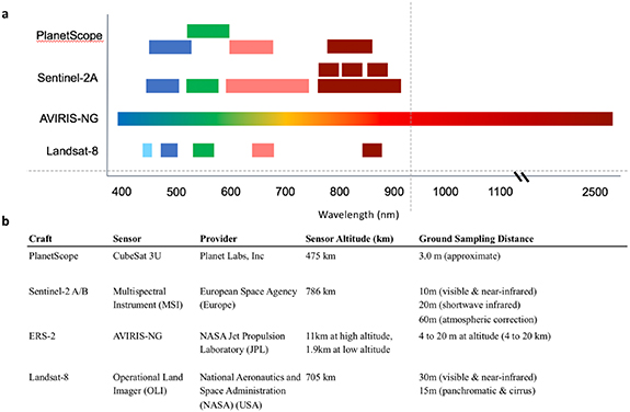
Figure 2. (a) Bandpass wavelengths (nm) in the visible bands and near-infrared for each sensor used in this study. The colors show the electromagnetic spectrum from blue (∼400 nm) to near-infrared (dark red, >700 nm). (b) Mission specifications for satellite and airborne imagery used in this study (b).
Download figure:
Standard image High-resolution imageAs part of the ABoVE campaign, AVIRIS-NG imagery was acquired on July 22, 2018. Level-2 (L2) atmospherically corrected Rs (Bue et al 2015) was downloaded from https://avirisng.jpl.nasa.gov/dataportal/. Sentinel-2 acquisitions were identified and downloaded from the U.S. Geological Survey Earth Explorer (https://earthexplorer.usgs.gov/) and atmospherically corrected using the Land Surface Reflectance Code (LaSRC) (Vermote et al 2016). Sentinel-2 images were also corrected using the dark spectrum fitting (DSF) algorithm available in ACOLITE (Python Version 20 190 326.0), which is an open-source atmospheric correction tested successfully in coastal waters (Vanhellemont 2019). PlanetScope Level-2 products were identified using the Planet Labs API (Planet 2017) and a cloud-native, scalable workflow called SWEEP (John et al 2019). No cloud-free Landsat overpasses occurred during or close in time to field operations.
To utilize long-term Landsat records, we also calculated Landsat growing season composites, which is the per-pixel median greenness over the growing season (June, July and August). A common remote sensing tool used to quantify terrestrial productivity (Roy et al 2010), growing season composites provide a continuous, stable record of seasonal lake color. While Landsat overpasses are infrequent (16 d) compared to Planet (∼daily), the Landsat program has the longest global record of Earth observation with acquisitions initiated in the mid-1980s (Lymburner et al 2016), making it a powerful tool for historical analysis. For L8 composites, Collection 1 Level 2 Rs was accessed using Google Earth Engine. To generate seasonal composites, per-pixel median greenness was calculated from all cloud-free images acquired during the growing season (June 1–September 30) over the study area. With the exception of ACOLITE, all Rs products described above are derived using 6 SV-based approaches (Vermote et al 2006). For brevity only those results are shown in the main text, but ACOLITE results are given in figures S1–2 (available at stacks.iop.org/ERL/15/105001/mmedia), table S3.
2.4. In situ surface reflectance validation data
In order to verify in situ lake color, Rs (350–2500 nm) was measured at each lake center in 2018 (n = 7) using an ASD FieldSpec 4 High Resolution Spectroradiometer (3 nm and 8 nm resolution in VNIR and SWIR) (text S2). Above-water, in situ lake Rs was collected 3–5 d prior to overpasses because same-day in situ validation was not possible due to weather delays.
2.5. Combining field and satellite observations
Lake color was extracted for each sampling location from PlanetScope, Sentinel-2, Landsat-8 and AVIRIS scenes for each lake (n = 7) using Google Earth Engine (Gorelick et al 2017). A 3 × 3 pixel-wise box centered on field GPS coordinates was drawn for each lake and the median Rs within each box was extracted from the image in order to reduce bias introduced by spatial sampling (Pahlevan et al 2016). In the case of scenes overlapping above a site, the median value between scenes was extracted. Since sampling was done at lake centers, all selected pixels were open water. A restrictive F-mask filter was also used to confirm selected pixels were water (Zhu et al 2015). Lake color from each respective platform was then regressed against in situ GPP (n = 7) using a reduced major axis (RMA) type II regression (Python package plyr2, (Haëntjens 2018)). This same workflow was also used to extract lake color from Landsat seasonal composites (section 2.3) for the 2016 samples (n = 24). The regression model was used to create satellite-derived maps of GPP by taking the regression equation derived from the GPP ∼ greenness relationship observed in the 2018 field campaign and applying it on a per-pixel basis to Sentinel-2 imagery using the green band as the model input.
2.6. Comparing surface reflectance across sensors
In order to make hyperspectral lake color comparable to multi-spectral observations, in situ and AVIRIS-NG Rs was spectrally convolved to Sentinel-2 wavelengths as in (Pahlevan et al 2017):
where:
 : band center wavelength
RSR: spectral response factor
n: total number of hyperspectral band centers (i)
Median absolute percent different (MAPD) was used to compare sensor Rs:
 where x is sensor 1 and y is sensor 2. For decadal time series analysis (figure 4), the non-parametric Mann–Kendall estimator and Sen's Slope were used to determine whether there was a positive or negative trend in lake greenness and its significance. Thiel–Sen Slope was calculated using the Scipy Python-based scientific computing package (Virtanen et al 2020) and significance of the slope was determined using a Mann–Kendall test (Hirsch et al 1982).
3. Results and discussion
3.1. In situ lake GPP
In situ median GPP rates (table 2) were high at 9.72 mg O2 m−2 d−1 and spanned a wide range (interquartile range = 6.25 to 10.50 mg O2 m−2 d−1). In situ GPP is on the same order of magnitude as other free-water techniques estimating GPP (Solomon et al 2013). The rates observed here are higher than more dilute and often deeper boreal lakes (Ask et al 2012, Deininger et al 2017) and are consistent with the high productivity observed in shallow, macrophyte-rich lakes found in the northwestern Siberia lowlands (Manasypov et al 2014) and shallow lakes in the Mackenzie Delta (Squires et al 2009, Tank et al 2009).
3.2. Controls on lake color
Other influences on lake color must be ruled out in order to avoid applying this empirical method over-ambitiously. To this end, we characterized variables (table 2) known to influence lake color, including phytoplankton pigments, CDOM and turbidity (Aurin and Dierssen 2012). We observed relatively low phytoplankton biomass based on HPLC Chl-a pigment analysis (median = 3.4 m−1, interquartile range = 2.4–5.9 µg l−1) (table 1). Overall, this is consistent with a previous study of 129 Yukon Flats lakes (table S1) showing Chl-a was lower than expected based on nutrient availability (Heglund and Jones 2003). The relatively clear waters and high GPP observed here in the presence of low phytoplankton biomass suggest macrophyte production is driving lake GPP (Genkai-Kato et al 2012). One exception was YF17, where field observations of a bloom were confirmed by high HPLC-derived Chl-a (83.3 µg l−1)
Table 1. Sampling dates, coordinates and physical properties of study lakes sampled in situ in July 2018 for GPP, reflectance, dissolved organic matter composition and chlorophyll-a among others (section 2.2, text s1).
| Latitude | Longitude | Date Sampled | Depth (m) | Surface Area (km2) | |
|---|---|---|---|---|---|
| Boot (B) | 66.07404 | 146.27066 | 7/18/18 | 22.0 | 0.73 |
| Canvasback (CB) | 66.38303 | 146.35489 | 7/19/18 | 1.4 | 2.83 |
| Greenpepper (GP) | 66.09209 | 146.73557 | 7/18/18 | 10.3 | 0.97 |
| Ninemile (NM) | 66.18285 | 146.66376 | 7/17/18 | 1.8 | 3.33 |
| Scoter (SC) | 66.24241 | 146.39896 | 7/17/18 | 4.5 | 4.56 |
| YF17 (Y17) | 66.32072 | 146.27431 | 7/17/18 | 1.6 | 1.75 |
| YF20 (Y20) | 66.63715 | 145.77278 | 7/17/18 | 1.3 | 0.59 |
The majority of lakes were shallow (median depth of 1.6 m) (table 1), with light extending to epiphytic periphyton and aquatic macrophytes. One lake was >10 m deep; the depth, low GPP and low Chl-a (table 2) of this lake provided an end-point representative of the gradient in the area. Other studies have established that submerged and floating macrophytes reflect in the green (560 nm) and near-infrared (850–880 nm) (Silva et al 2008, Oyama et al 2015, Palmer et al 2015, Dogliotti et al 2018). The shallow depths of these relatively clear lakes, as inferred by low turbidities (<1 FNU in most cases) could allow signals from macrophytes and periphyton to reach the surface (Mobley et al 2020). Given the low Chl-a, low turbidities and the observed presence of macrophytes within the water column we suggest that overall, phytoplankton production is not a significant component of the optical signature.
Table 2. Limnological conditions for Yukon Flats sites sampled in 2018. Values given represent the means and, when more than two replicates were collected, standard deviations of the replicates are given as well.
| pH | Turbidity (FNU) | Chl-a (μg l−1) | GPP (g O2 m−2 d−1) | a440 (m−1) | DOC (mg l−1) | ||
|---|---|---|---|---|---|---|---|
| Boot (B) | 8.31 | 0.54 | 2.7 ± 0.05 | 3.0 | 1.2 ± 0.12 | 19.2 ± 0.21 | |
| Canvasback (CB) | 9.55 | 0.96 | 2.26 ± 0.01 | 10.7 | 2.41 ± 0.17 | 29.83 ± 0.22 | |
| Greenpepper (GP) | 9.02 | 0.96 | 4.1 ± 0.04 | 6.2 | 0.42 ± 0.03 | 32.82 ± 0.40 | |
| Ninemile (NM) | 9.46 | <0 | 6.5 ± 0.00 | 9.7 | 1.09 ± 0.31 | 27.64 ± 0.07 | |
| Scoter (SC) | 8.93 | <0 | 7.1 ± 0.05 | 6.3 | 0.47 ± 0.20 | 19.46 ± 0.08 | |
| YF17 (Y17) | 9.82 | 35 | 83.3 ± 0.33 | 14.6 | 2.42 ± 0.59 | 35.65 ± 0.54 | |
| YF20 (Y20) | 10.24 | <0 | 1.26 ± 0.4 | 10.3 | 1.09 ± 0.83 | 10.17 ± 0.14 | |
A second influence on lake color is absorption of light by CDOM. CDOM can interfere with the remote sensing of GPP in two ways. CDOM absorbs green light, so high CDOM has the direct effect of masking green light reflected from photosynthetic pigments (Carder et al 1989). Indirectly, CDOM can shade out aquatic producers, thus having the ecological impact of reducing GPP (Ask et al 2012, Seekell et al 2015). In order to rule out this influence, CDOM data were collected at each site. CDOM values (table 2) in sampled lakes were low (a440, median = 1.13 m−1, interquartile range = 0.78–1.82 m−1), showing that lakes are relatively clear despite their high DOC (10.2 to 25.6 mg l−1) (table 2). Our findings are consistent with other studies in semi-arid aquatic ecosystems (Osburn et al 2011, Bogard et al 2019, Kellerman et al 2019) that show low CDOM despite high DOC. While coupling between DOC and CDOM has been demonstrated at global scales (Massicotte et al 2017), CDOM-DOC decoupling in these semi-arid landscapes is hypothesized to result from decreased hydrologic connectivity which reduces terrestrial organic carbon subsidies as aromatic carbon compounds to aquatic ecosystems, resulting in clearer lakes than otherwise expected (Johnston et al 2020).
Finally, lake color can be influenced by scattering from sediment during periods of hydrologic connectivity to surface waters or during lake turnover. However, turbidity across lakes was low (<1 FNU) (table 2) with the exception of YF17, where the previously noted algal bloom drove turbidity up to 35 FNU. Taken together, these results indicate the clear and shallow nature of these macrophyte-rich lakes creates favorable conditions for the remote sensing of benthic properties.
3.3. Linking in situ GPP to Sentinel-2 lake color
Lake color from satellite and airborne sensors was regressed against 2018 in situ GPP (mg O2 m−2 d−1) (n = 7), revealing a strong, positive correlation between greenness and GPP (figure 3(a), p-value < 0.05). We then applied this regression pixel-wise to Sentinel-2 imagery to create spatially explicit GPP maps (figures 3(b) and (c)) for each lake. Modeled, S2 GPP ranged from 3.9 ± 1.14 mg O2 m−2 d−1 in the deep, upland Boot Lake to 14.21 ± 6.42 mg O2 m−2 d−1 in shallow, eutrophic YF17.

Figure 3. (a) Scatterplot showing the relationship between GPP measured in situ in 2018 and greenness as derived from Sentinel-2 surface reflectance (∼560 nm) for July 2018 lake samples (n = 7). The equation shown in figure 3(a) was then applied per pixel to the Sentinel-2 imagery, resulting in spatially-explicit maps of GPP. Examples of these resulting GPP maps modeled from satellite imagery are shown for two of the study lakes: (b) Canvasback Lake and (c) Scoter Lake. The color bar indicates the range of values for modeled GPP derived by applying the equation in figure 3(a) to each Sentinel-2 pixel.
Download figure:
Standard image High-resolution image3.4. Independent evaluation with Landsat
The relationship was then evaluated using a separate dataset from a 2016 field campaign that had been withheld for independent testing (figure 4). As same-week images were not available, we instead regressed seasonal L8 composites against 2018 (n = 7) and 2016 in situ GPP (n = 17) (Bogard et al 2019). The correlation between greenness and in situ GPP was maintained across both models.
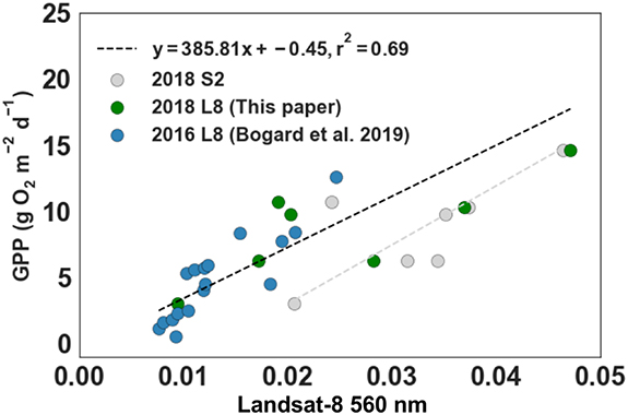
Figure 4. Scatter plot using L8 composites (Rs; 560 nm) and in situ GPP from 2016 and 2018 (g O2 m−2 d−1) (n = 24). The 2016 in situ GPP is the average of June and September; 2018 in situ GPP was collected once during July. The 2016 (shown in blue, n = 17) and 2018 (shown in green, n = 7) Rs was calculated from June to September composites (see text for full description). The S2 model from figure 1(d) (n = 7) is shown in grey for comparison. L8 regression model and coefficients of determination (r2) are given in inset. Scene IDs can be found in table S2.
Download figure:
Standard image High-resolution imageThe L8 seasonal composites produced a slightly stronger relationship (type 2 major axis regression: y = 385.81x−0.45; r2 = 0.69; p = 2.60 × 10⁻⁴, n =24) than the Sentinel-2 same-week model. This likely results from the smoothing of short-term variability from the composite and the relative stability of oxygen pools (Bogard et al 2017) in these shallow lakes on seasonal scales. The separate models provide an independent check against each other, further substantiating the robustness of this approach across sensors and years.
The use of Landsat allows us to tap into the powerful historical imagery available through the Landsat archive in order to detect decadal (Wang et al 2014, Lymburner et al 2016) and seasonal (Kallio et al 2008) trends in lake color. Lake greenness computed for Scoter Lake (figure 5) showed a decline from 1984 to 2018. Field studies suggest that declines in greenness could result from increased CDOM absorption resulting from thermokarst processes for lakes with higher absorption (Wauthy et al 2018), increases in depth (Duguay and Lafleur 2003), or increased sediment loading during periods of surface water connectivity (Vonk et al 2015). Subsequent research combining these techniques with paleolimnology (Pienitz et al 1999, Bouchard et al 2017) and radiocarbon (Rühland et al 2003) data has the potential to unveil past lake processes, although more testing is required to establish mechanistic links between these processes and lake color across more diverse ecosystems.
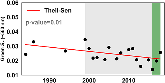
Figure 5. Landsat time series of greenness for Scoter Lake. Black dots represent median growing season greenness at the sampling location. The red line is the Thiel–Sen slope (y = −0.00023x + 0.61) with the p-value from the Mann–Kendall significance test given top left. Grey shading depicts launch of Landsat-7, after which two Landsat sensors have continuously been in orbit. Green shading represents time period of ABoVE field campaigns.
Download figure:
Standard image High-resolution image3.5. AVIRIS-NG, PlanetScope and in situ Rs
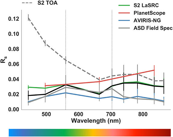
Surface reflectance from different sensors showed the greatest agreement in the green band.
Using high-resolution PlanetScope and AVIRIS-NG Rs (table S2), Sentinel-2 and in situ Rs (figures 6, S1-2), we compared Rs and respective model performance using 2018 in situ GPP. Analyzing agreement between the blue, green, red and NIR bands, we found the best agreement in the green (MAPD median = 29%, interquartile range 8%–53%) (figure S1-2, text S3-4).
Figure 6. Surface reflectance (Rs) represented as the median and interquartile range (25%, 75%) of 2018 lakes. Dashed vertical grey lines show the wavelengths used to model GPP at 560 nm (green) and 704 nm (red-edge). S2 TOA spectra given for context. Extended discussion of differences given in text S3 and figure S2. It is important to note ASD measurements (table 1 for dates) were collected prior to airborne (July 22) and satellite (PlanetScope, July 23; Sentinel-2, July 22) measurements.
Download figure:
Standard image High-resolution image
Green Rs is less subject to inter-sensor differences (Pahlevan et al 2018) and calibration errors between Landsat sensors (Vogelmann et al 2016). S2's green Rs has been successfully ground-truthed over small thermokarst lakes and ponds by Freitas et al (2019) and green Rs is also less impacted than NIR by particulates (Wang and Philpot 2007). Green Rs also has the major advantage of being measured by almost every spectral remote sensing platform, dating back to early Landsat (Dwyer et al 2018) and including the upcoming Plankton Aerosol, Cloud, Ocean Ecosystem (PACE) Mission (Werdell et al 2019). Finally, previous studies have shown greenness covaries with both phytoplankton (O'Reilly et al 1998, O'Reilly and Werdell 2019) and macrophytes (Hestir et al 2015). In light of the larger disagreements between sensors detected in the NIR (text S4), these results suggest that green Rs may be a stable, sensor-agnostic quantity suitable for GPP modeling across a range of spectral, spatial and temporal resolutions.
3.6. GPP model results for green and red-edge bands across sensors
In situ GPP (mg O2 m−2 d−1) corresponded with greenness (table 3, figures S3–4). The strongest correlation was between in situ GPP and in situ Rs (r2 = 0.68; p-value < 0.05) and CubeSat Rs (r2 = 0.78; p-value < 0.05). This could be due to two factors. First, in situ Rs was collected simultaneous to in situ GPP, in contrast to the overpasses 2–5 d later. However, unlike dynamic river and coastal systems, processes in these lakes vary on seasonal and annual scales. For example, high-frequency daily observations of dissolved oxygen collected from May to September (Bogard et al 2019) show consistently positive rates of net production driven by intense plant growth was sustained throughout most of the growing season. Johnston et al (2020) also showed diel dissolved organic matter composition and optical properties changed minimally over a 3 d period. A second reason for the stronger performance of PlanetScope and the in situ sensor's performance could be because of their finer spatial resolution relative to other sensors (10–30 m).
Table 3. Regression results between July 2018 Rs and in situ GPP fitted using a Type II regression model using the green (560 nm) and the red-edge (704 nm) bands from each sensor. The empty row results from PlanetScope lacking a red-edge band. All p-values were <0.05 (table S3) and individual scatterplots are provided in figures s3 and s4.
| Green (∼560 nm) | Red-edge (∼704 nm) | |||||
|---|---|---|---|---|---|---|
| Slope | Intercept | r2 | Slope | Intercept | r2 | |
| S2 TOA | 478.91 | −22.46 | 0.30 | 478.91 | −22.46 | 0.56 |
| S2 LaSRC | 446.18 | −5.93 | 0.53 | 446.18 | −5.93 | 0.62 |
| PlanetScope | 413.39 | −6.65 | 0.78 | NA | NA | NA |
| AVIRIS-NG | 607.19 | −4.51 | 0.40 | 607.19 | −4.51 | 0.74 |
| ASD Field Spec | 146.86 | 4.43 | 0.68 | 146.86 | 4.43 | 0.80 |
While restricting the time difference between field and satellite observations can improve model uncertainty in dynamic river systems (Kuhn et al 2019), albeit time differences of up to 3 to 5 d have been used successfully in several lake studies (Kloiber et al 2002, Chipman et al 2004, Olmanson et al 2008, Boucher et al 2018). Shorter time differences are ideal, yet given the temporal stability of the dissolved oxygen pool and water color over several days in these lakes, we are confident that these results are representative and provide important insights, particularly given the lack of comparisons of surface reflectance over inland waters (Maciel et al 2020).
A second advantage of Sentinel-2 over Landsat-8 is the addition of red-edge bands suitable for mapping vegetation. An even stronger correlation than with greenness was observed between GPP and the red-edge band (704 nm) (table 3, S3). Models improved by an average of 16% (table 3) due to the strong red-edge reflectance of macrophytes. This suggests that, when available, red-edge bands may be the strongest candidate for modeling GPP in these shallow lake ecosystems whose GPP is driven by both macrophytes and phytoplankton. This finding has implications for future missions as red-edge bands with narrower bandpasses are increasingly being added to, for example, Planet Lab's next-generation Dove satellites. While the green band is suitable for historic analysis, these findings encourage red-edge based algorithm development due to the strong signal in these shallow arctic and boreal lakes.
The correlation between green and NIR bands with in situ GPP across sensors and sites indicates their potential as a simple GPP proxy for shallow lakes with low turbidity and CDOM. For context, global ocean models typically only explain 40% of water-column-integrated primary production (Siegel et al 2001). The strength of this relationship between lake color and in situ GPP for both 2016 and 2018 datasets suggests potential for the development of a remote sensing modeling framework for shallow lake GPP.
4. Conclusions
This study provides evidence of a simple empirical relationship between lake color and GPP for shallow, relatively clear boreal lakes using in situ field data paired with remote sensing. We use a novel approach that pairs oxygen isotopes with satellite imagery. Both techniques integrate pelagic and benthic processes from phytoplankton and macrophytes in shallow waters (Wetzel and Hough 1972, Jackson 2003). Summertime CO2 drawdown in shallow lakes has been linked to macrophyte growth, highlighting the potentially important role of macrophytes in lake carbon cycling (Tank et al 2009, Vesterinen et al 2016). Shallow lakes are abundant worldwide and therefore the ability to integrate benthic and pelagic GPP is crucial for capturing whole ecosystem GPP.
In terrestrial systems, NDVI has been widely adopted as a useful, albeit imperfect, proxy for vegetation biomass (Rouse 1974). NDVI has transformed our understanding of landscape change in remote northern regions (Jia et al 2003, Goetz et al 2005, Bhatt et al 2013, Ju and Masek 2016, Sulla-Menashe et al 2018), yet no such metric has been adopted for shallow lakes. This study provides initial evidence of the green band as a potential simple index for mapping GPP in shallow, light-filled, and highly productive northern lakes. We then confirmed this relationship using Landsat-8 and compare results from other sensors including AVIRIS-NG and PlanetScope. This study demonstrates green and red-edge bands from Sentinel-2, Landsat-8, AVIRIS-NG and PlanetScope can be used to map GPP when constrained with appropriate field data. More detailed in situ measurements of lake color and biogeochemistry across optically diverse systems are needed to further test this finding. Advances in field data collection needs to be prioritized for algorithm development across the circumpolar north.
In the Yukon Flats, warming and thawing has led to lake area decline (Jepsen et al 2013, 2016). Surveying all 30 000 lakes in this region is not feasible yet the area is predicted to undergo drastic hydrologic changes linked to increasing permafrost thaw (Walvoord and Striegl 2007, Walvoord et al 2012). Our findings suggest further work developing remote sensing algorithms for GPP could advance lake monitoring at scales useful for climate science and ecosystem management.
Acknowledgments
This research was supported by a NASA Earth and Space Science Fellowship (NESSF) awarded to CDK. Data collection was also supported by NASA-ABoVE Project 14-14TE-0012 (awards NNH16AC03I and NNX15AU14A) and the U.S. Geological Survey (USGS) Land Carbon Program. Sample collection was made possible by the expert flights in and out of lakes by Jim Webster (Webster's Flying Service). We thank the Remote Sensing and Geospatial Analysis Laboratory (RSGAL) lab for the use of the ASD Field Spectrometer. Any use of trade, firm, or product names is for descriptive purposes only and does not imply endorsement by the U.S. Government. We also thank three anonymous reviewers for their constructive comments.
Data availability statement
Any data that support the findings of this study are included within the article.