

Abstract
Climate services that can anticipate crop yields can potentially increase the resilience of food security in the face of climate change. These services are based on our understanding of how crop yield anomalies are related to climate anomalies, yet the share of global crop yield variability explained directly by climate factors is largely variable between regions. In Europe, France has been a major crop producer since the beginning of the 20th Century. Process based and statistical approaches to model crop yields driven by observed climate have proven highly challenging in France. This is especially due to a high regional diversity in climate but also due to environmental and agro-management factors. An additional level of uncertainty is introduced if these models are driven by seasonal-to-decadal surface climate predictions due to their low performances before the harvesting months of both wheat and maize in western Europe. On the other hand, large scale circulation patterns can possibly be better predicted than the regional surface climate, which offers the opportunity to rely on large scale circulation patterns as an alternative to local climate variables. This method assumes a certain degree of stationarity in the relationships between large scale patterns, surface climate variables, and crop yield anomalies. However, such an assumption was never tested, because of the lack of suitable long-term data. This study uses a unique dataset of subnational crop yields in France covering more than a century. By calibrating and comparing statistical models linking large scale circulation patterns and observed surface climate variables to crop yield anomalies, we can demonstrate that the relationship between large scale patterns and surface variables relevant for crop yields is not stationary. Therefore, large scale circulation pattern based crop yield forecasting methods can be adopted for seasonal predictions provided that regression parameters are constantly updated. However, the statistical crop yield models based on large-scale circulation patterns are not suitable for decadal predictions or climate change impact assessments at even longer time-scales.
Export citation and abstract BibTeX RIS

Original content from this work may be used under the terms of the Creative Commons Attribution 4.0 license. Any further distribution of this work must maintain attribution to the author(s) and the title of the work, journal citation and DOI.
1. Introduction
Global agricultural crop areas have been increasingly exposed to unfavourable weather conditions, significantly deteriorating yields of the main agricultural crops (Lesk et al 2016, Zampieri et al 2017a). Climate change is expected to exacerbate the frequency, severity, and spatial extent of extreme events (Zhu and Troy 2018, Ceglar et al 2019, Zampieri et al 2019) thereby changing the risk of simultaneous breadbaskets failures (Gaupp et al 2020). Preventing adverse effects of unfavourable climate events on crop yields to avoid crop failures requires timely and effectively planned agronomical decisions, which can be put in practice if the future weather evolution is known early enough in the growing season. As the location and magnitude of surface weather anomalies are difficult to predict beyond a two weeks horizon, understanding the relationship between large-scale atmospheric circulation patterns and surface climate variability (including extremes) might provide a more effective way to predict the potential impact on crops. Relevant dynamical processes on sub-seasonal to seasonal time scale include features such as El-Nino (Cane et al 1994, Iizumi et al 2014), Madden and Julian oscillation (Andersson et al 2020), stratospheric circulation (Byrne et al 2017), stationary Rossby waves (Kornhuber et al 2019), and large-scale atmospheric circulation patterns (Ceglar et al 2017). In this study, we focus on the latter.
Europe is predominantly influenced by four large-scale atmospheric circulation (hereafter LS) patterns: the North Atlantic Oscillation (NAO), the East Atlantic (EA), the East Atlantic-West Russian (EAWR) and the Scandinavian (SCAND) patterns (Gonzalez-Reviriego et al 2015). Large-scale atmospheric circulation in the Euro-Atlantic region has an important control over the regional surface climate in Europe (Bladé et al 2012, Toreti et al 2010, Casanueva et al 2014, Krichak et al 2014, Ceglar et al 2017). The persistence of certain types of circulation patterns is associated with the occurrence of anomalous well-characterized spatial patterns of climate conditions; for example, NAO has been shown to have a strong influence on drought variability across Europe (e.g. van der Schrier et al 2006, Vicente-Serrano et al 2016).
LS patterns have been shown to control vegetation activity in Europe, with the CO2 land sink being influenced by NAO and EA coupling (Maignan et al 2008, Bastos et al 2016). The signature of these climate features has been identified in complex biophysical variables such as crop yields (e.g. Sepp and Saue 2012, Brown 2013, Irannezhad and Klöve 2015, Ceglar et al 2017). LS patterns have been shown to account for up to 70% of inter-annual crop yield variability in Europe (Cantelaube et al 2004, Ceglar et al 2017). Identification of precursor mechanisms leading to potential negative crop yield anomalies at harvest can effectively provide an early warning for adapting agro-management decisions with beneficial economic prospects for farmers (Faloon et al 2018). The recent improvements in predictability of large scale atmospheric circulation over the Euro-Atlantic region, with key factors such as the winter NAO being predictable months ahead (Scaife et al 2014, Dunstone et al 2016), provide an opportunity to use skilful seasonal forecasts for improved yield forecasts.
To benefit from seasonal climate predictability, it is important to understand the link between LS patterns and yields. Such relationships have been explored and established for agriculture (e.g. Ceglar et al 2017, Heino et al 2018, Nobre et al 2019) and wind energy (e.g. Ely et al 2013). The impact of LS patterns is indirect through their effect on regional surface climate. Understanding the relationship between LS and complex biophysical variables, such as crop yield, is complicated by the time-varying LS impact on surface regional climate, and lagged responses of ecosystems through phenology and soil moisture carry-over effects (Bastos et al 2016). The formation of yield may be sensitive to specific conditions during grain filling that can be connected to the previous growing season such as the occurrence of diseases (Capa-Morocho et al 2014, Caube et al 2017, Ben-Ari et al 2018). Additionally to the climatic fingerprint, the inter-annual variability and trends of crop yields can be influenced by human intervention (such as reactive in-season agro-management and irrigation practices, and more gradual changes in characteristics and choice of crop varieties).
The impact of LS patterns on regional surface climate in Europe is characterized by nonstationarity, which is likely linked to interdecadal shifts in the locations of the LS pressure centers (Vicente-Serrano and Lopez-Moreno 2008). However, stationarity is often assumed for empirical relationships between LS and crop yields due to short historical yield records that limit a more formal analysis. The temporal evolution and magnitude of LS circulation impact on crop yields are important to better understand past regional co-variability between climate and crop yields and have clear significance for impact assessments at seasonal and/or decadal time scales. This study aims to identify those LS patterns with significant impact on crop yields on centennial time scale and to discuss the temporal variation of these impacts. Furthermore, we do so at subnational level to capture the spatio-temporally evolving regionally diverse impacts of LS patterns on surface climate across France. For this purpose, we derive and apply a statistical framework linking LS patterns and regional surface climate to a long-term record of French soft wheat and maize yields starting in 1900.
2. Data and methods
2.1. Crop yield data
Crop yield, production and areas on regional (department) level from 1900 until 1988 in France were collected from books of national agricultural statistics ('Statistique agricole annuelle' or 'Annuaire de statistique agricole') and merged together with crop yield data from the Agreste website (agreste.agriculture.gouv.fr; 'Statistique agricole annuelle') for the period between 1989 until 2016. Following (Schauberger et al 2018) we use here the 96 French mainland departments in their current form, which is an equivalent to NUTS3 administrative division (figure S2 (available online at stacks.iop.org/ERL/15/094039/mmedia)). Since the shapes of French departments have changed over time, the historical yield values were subsumed to modern departments. Crop yields were calculated from total production and surface area for each department.
The two main crops grown in France have been analysed in this study: soft wheat and grain maize. The manual digitization of data points from statistical yearbooks was a large effort subject to possible errors. Hence, to evaluate the quality of the database, a preprocessing of the crop yield data is necessary. Apart from physiologically unattainable values, abrupt changes in time series within one department are considered as possible reporting errors. These latter values are detected by the defined 99% quantile and standard-deviation filters. Though this automatic filter procedure may indeed remove some correct values, we assume that the alternative of manual filtering by an expert would be more subjective (and not feasible given the large amount of data). The following quality filters have therefore been applied to check for digitizing errors in time series of crop yield figures:
- (i)unreasonable absolute values larger than a physiologically currently unreachable yield (20 t ha−1 for maize and wheat) are removed,
- (ii)the top 1% of values across all departments per decade are removed,
- (iii)values deviating more than four standard deviations around the mean of each crop-department time series (for yield, area or production) are removed, and
- (iv)a similar thresholding approach is applied within each decade of a single time series (for yield, area or production), filtering values above or below decadal mean ± two (yield) or three (area, production) decadal standard deviations.
figures 1(b) and (c) shows the resulting time series of total soft wheat (sum of winter and spring soft wheat) and grain maize yields, aggregated at national level.

Figure 1. (a) Time series of first four leading modes of large-scale atmospheric circulation patterns over the euro-atlantic region since 1901 (NAO, EA, EAWR and SCAND). (b) The time series of total soft wheat yield on national level since 1901 (black line). Detrended yields (using dynamic linear model) are denoted by red line, while dashed blue line (belonging to secondary axis) represents the yield standard deviation calculated using a moving window of 40 years. (c) Same as (b) but for grain maize.
Download figure:
Standard image High-resolution image2.2. Time series of large-scale circulation patterns
The time series of the four main Euro-Atlantic LS patterns (NAO, EA, EAWR and SCAND) for the period 1901–2010 have been obtained from the 500-hPa geopotential height (Z500) of the 20CR version 2 reanalysis (Compo et al 2011) through the application of the Partial Least Squares (PLS) regression, as described in Gonzalez-Reviriego et al (2015). The main advantage of using the PLS regression, in comparison with the traditional EOF or REOF methods, is the higher correspondence obtained for the common period 1950–2000 between the 20CR time series of the LS patterns and those monitored by the National Oceanic and Atmospheric Administration (NOAA) Climate Prediction Center (CPC). In the PLS regression, the four LS spatial patterns (NAO, EA, EAWR and SCAND) monitored by NOAA-CPC for the period 1950–2000, have been used as dependent variables and the 20CR Z500 anomalies for the period 1901–2010 as explanatory variables. Since neither the dependent or explanatory input variables are standardized (both are given in the spatial domain), the obtained PLS regression coefficients were standardized for the period 1981–2010, which is the reference period used by CPC to normalize the time series of the LS patterns. Standardized regression coefficients obtained in this way represent the time series of the Euro-Atlantic LS patterns for the 20CR reanalysis. This procedure is applied for each season (DJF, MAM, JJA and SON) separately (figure 1(a)).
2.3. Observational gridded weather data
The Climate Research Unit (CRU) gridded climate dataset (version 4.03) is used here to obtain data on monthly average temperature and precipitation cumulates (Harris et al 2014). The CRU data represents gridded fields based on monthly observational data calculated from daily or sub-daily data by National Meteorological Services and other external agents. The resolution of the grid is 0.5° and covers a period between 1901 and 2016. Gridded temperature and precipitation data over France have been aggregated to French department levels.
2.4. Empirical relationship between climate and crop yields
To establish the empirical relationship between LS circulation patterns and crop yields, a similar methodology has been followed as in Ceglar et al (2017). The steps followed in this analysis are presented in a schematic workflow in figure S1.
A multi-decadal trend in crop yield time series can be induced by the combined effects of changes in agro-management practices, environmental and socio-economic factors and climatic changes. The climate factors can have a significant influence not only on interannual yield variability but also on its long-term trend. Agnolucci and De Lipsis (2020) have shown that the trend in temperature is responsible for a reduction in the long-term growth rate of wheat yields in major European wheat producing countries. Nevertheless, since our focus is on the inter-annual crop yield variability, the multi-decadal trend in time series is first removed using Dynamic Linear Models (DLMs). In statistical literature the DLMs might go by a different terminology; in Harvey (1991) they are called structural time series. The DLMs are a type of linear regression models with time-varying rather than fixed parameters and were shown to be a robust method for crop yield trend analysis (Michel and Makowski 2013). In our study, the DLMs are applied for each crop and each department to detrend crop yield time series (see Schauberger et al 2018, for more details).
Detrended yield data are then used to build the main statistical models at department level:

where  represents detrended crop yield anomaly in year t,
  the explanatory variables (seasonal NAO, SCAND, EA and EAWR values) in year t and
  is the residual term. The growing period for soft wheat starts in autumn and finishes in the summer of the following year. Spring, summer and autumn are considered as potential explanatory seasons for grain maize. The empirical regression models are derived for moving 40-year periods, starting with the period 1901–1940 (figure S1). Linear detrending is applied to all explanatory variables (LS patterns) for each time window of 40 years. Crop yields and explanatory variables are also standardized (mean = 0 and std = 1) for each period; the standardization makes the regression results comparable between different regions and time periods considered. The normality of derived model residuals has been tested using the Shapiro test, while the Durbin-Watson test has been used to detect the presence of autocorrelation in residuals (Wilks 2006).
Initially, all explanatory variables are included in the regression model (figure S1). For total soft wheat, these amount to 16 variables (4 LS patterns for each season), while this amounts to 12 variables for grain maize. Regularization is therefore necessary to reduce the model to the most important variables and to reduce multicollinearity between the independent variables. For this purpose, all explanatory variables are first included into a Least Angle Regression Scheme (LARS; Efron et al 2004) to evaluate and rank those variables contributing the most to the variance of the predicted yield. LARS is a model-selection method, providing an ordering in which the covariates enter the regression model. The main principle of the LARS is to add or drop covariates one-at-time; coefficients are updated at each step in equiangular direction of the most correlated covariates until a new covariate is added or dropped. To increase the robustness of the method in the presence of outliers, we use the robust LARS (RLARS), where the classical correlations between covariates are replaced by robust correlation estimates (Khan et al 2007). Finally, we generate bootstrap samples on the original data and apply RLARS on each of these samples to sequence predictors. The predictors are then ranked according to their average rank over the bootstrap samples. The final set of ranked predictors is chosen by minimizing the corrected Akaike Information Criterion (AICc; Hurvich and Tsai 1991).
After the final set of predictors is identified based on the above procedure applied for each department, the regression model (1) is then used again with the identified set of predictors to derive department-based standardized regression coefficients. The significance of derived department-based regression models is assessed using the p-values obtained by an F-test. To account for multiple hypothesis testing (i.e. false detection rate) for 96 departments, individual significance tests on department level are corrected using the procedure proposed by (Strimmer 2008).
The above procedure to establish department-level regression models is followed also using surface climate as explanatory variables (replacing the LS patterns in equation (1) with seasonal averages of temperatures and cumulates of precipitation). However, in this case the number of explanatory variables is lower, initially amounting to 8 variables for soft wheat and 6 for grain maize (figure S1).
3. Results
3.1. Time-varying impact of climate on soft wheat yields
Figure 2(a) shows the time series of obtained regression coefficients for total soft wheat together with the share of affected crop area at national level. The regression coefficients are calculated using predictors and explanatory variables on the moving window of 40 years; the coefficients displayed represent the central year of each moving window. Winter EAWR and spring EA patterns influenced the highest share of soft wheat cropland during the first half of the 20th Century; but their influence gradually decreased during the second half of the 20th Century. While the impact of positive spring EA on yield remains negative through the entire period of analysis, the standardized regression coefficient of winter EAWR pattern reverses sign in the 1980's. This is also visible on figure S2(a), showing regional regression coefficients for three different periods. The strong positive impact of EAWR during the winter in a major part of France gradually weakened and even reversed its sign in the most recent period. A noticeable feature is an increase in influence of the autumn SCAND pattern after mid-century, however with high inter-annual variations in the area affected. SCAND influenced wheat in a major part of France, except for the Mediterranean and eastern continental regions during the 1941–1980 period (figure S2(a)). Its influence has been weakening towards the end of the analysed period. During the recent period the impact of spring SCAND pattern and summer EA pattern is observed, with positive phases of both related to positive crop yield anomalies.

Figure 2. (a) Standardized regression coefficients of the four leading atmospheric modes of variability for regional-based total soft wheat yield regression models. The regression models are derived for each department separately, followed by aggregation of their predictions to national level using a wheat area weighted average. For each year the regression coefficients are calculated using predictors and explanatory variables on the moving window of 40 years. The coefficients displayed represent the central year of each moving window (e.g. coefficients displayed for 1960 are derived from data between 1941 and 1980). The size of the circle denotes the share of wheat area affected by large scale atmospheric circulation (i.e. cumulative area where obtained regression models are significant, p < 0.05). Grey colour represents non-significant regression coefficients. (b) Same as a) but using seasonal precipitation cumulates and average temperature as explanatory variables. The size of the circle denotes the share of wheat area affected by seasonal temperature and precipitation (i.e. cumulative area where obtained regression models are significant, p < 0.05).
Download figure:
Standard image High-resolution imageFigure S2(b) shows regression coefficients obtained for winter soft wheat only, calculated for the period after 1960 due to the lack of separation in reported winter and spring soft wheat statistics before the 1950s. The comparison of coefficients with those in figure 2(a) shows very little differences, indicating that total soft wheat inter-annual variability is mainly governed by winter soft wheat. This is confirmed also by correlation figures between the total soft wheat yields and winter soft wheat yields, which almost equals 1 (Schauberger et al 2018).
Large scale atmospheric circulation has only an indirect impact on crop yields through controlling regional surface climate. To elucidate the role of temperature and precipitation directly, we also derive empirical relationships between these regional surface climate variables (mean seasonal temperature and precipitation cumulates) as predictors for crop yield anomalies. The results exhibit similarity to the decreasing influence of winter LS circulation on wheat yields; a decrease of winter temperature and precipitation impact can be observed in the second half of the 20th Century (also in terms of total soft wheat area affected). Negative regression coefficients related to winter precipitation indicate a deteriorating influence of positive rainfall anomalies on wheat especially during the first half of the 20th Century. Similar to winter EAWR, the impact of winter temperature reverses its sign in the second half of the 20th Century. Another interesting feature can be observed in terms of summer temperature and precipitation; while the regression coefficients are negative throughout the entire analysed period, their amplitude strengthens after the 1950s. This indicates an increasingly negative impact of positive temperature and precipitation anomalies during the summer.
3.2. Time-varying impact of climate on grain maize yields
Grain maize has been mostly affected by the summer LS patterns (figure 3). The two most important modes of LS variability in this case are summer SCAND and summer NAO patterns. Summer SCAND affected a major proportion of maize cropland in France until the late 1960s, when the impact started to decrease sharply. Since the 1950s the summer NAO became the most prominent mode affecting maize yields in France (together with summer EAWR after 1980s).
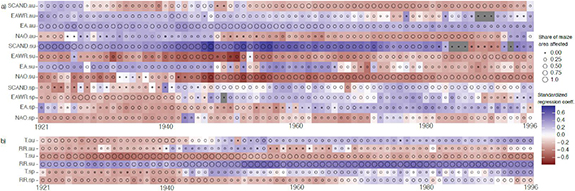
Figure 3. As figure 2, but for grain maize.
Download figure:
Standard image High-resolution imageRegression coefficients obtained from surface climate exhibit similar patterns of change; summer rainfall became more important in the second half of the Century. Nevertheless, its relevance is slightly decreasing towards the end of the analysed period. Summer temperature affected large maize areas at the beginning of the 20th Century, followed by a period of little influence from mid-Century until the 1990s after which it started to affect large areas of maize again. Surface climate in spring and autumn had only limited effect across the country.
3.3. Temporal evolution in explained variability of crop yields
The obtained regression models are able to explain a higher share of observed inter-annual crop yield variability at the beginning of the 20th Century (figures 4(a) and (c)). A distinctive drop in explained variance can be observed roughly between the 1950s and 1980s for total soft wheat, followed by an increase after the 1980s. Models based on regional surface climate (seasonal mean temperature and precipitation cumulates) generally explain more variability in observed wheat yields than the LS counterpart until the 1980s, when seasonal LS circulation becomes a stronger predictor than surface climate. Contrarily, surface climate predictors are able to explain more variability than LS predictors for grain maize during the entire analysed period (figure 4(c)). Reconstructed yields of total soft wheat and grain maize (figures 4(b) and (d)) show the lack of both regression approaches to capture the magnitude of lower yield anomalies, especially after the 1960s.

Figure 4. (a) Explained variability of soft wheat yields (winter, spring and total soft wheat yields) obtained by deriving the moving window regression models (using a time window of 40 years). (b) Reconstructed total soft wheat yield anomalies. Black lines represent standardized measured yield. Green lines represent results obtained by using large scale atmospheric indicators as predictors, while blue lines represent results obtained by using surface meteorological variables as predictors. The shaded area around green and blue lines for each year denotes the range of predictions of the entire set of regression models from the moving window of 40 years that include that specific year in the calibration (e.g. yield anomaly in year 1950 is predicted using 40 different derived regression models from the moving time window). The uncertainty range diminishes at the beginning and at the end of time series, where the first year (1901) and last year (2016) are used only once to derive the first and last regression model from the moving time window. (c) Same as (a), but for grain maize. (d) Same as (b), but for grain maize.
Download figure:
Standard image High-resolution image4. Discussion
4.1. Underlying reasons for varying impact of surface climate on crop yields
4.1.1. Grain maize.
Our analysis for grain maize shows that it is primarily sensitive to summer climate anomalies. Reduced sensitivity to summer temperatures after the 1960s could be related to improved crop management and an increasing share of irrigated cropland in France. The cropland area equipped for irrigation, which was below 0.5 Mha before the 1960s, thereafter sharply increased to above 2.5 Mha at the beginning of the 21st Century (Siebert et al 2015, Schauberger et al 2018). By 1975, maize was occupying roughly 35% of irrigated cropland in France (OECD 2000); before that, maize was likely much less irrigated, as irrigation traditionally was used for market gardening and horticulture as well as orchards (OECD 2000). The share of both maize harvested area and cropland irrigation extent have increased after the 1960s; nearly 50% of maize was irrigated at the beginning of the 21st Century. Notwithstanding this, the increasing sensitivity to summer temperature after the 1990s has likely been caused by increasing occurrence of heat stress and reduced grain filling length, confirming previous results of Ceglar et al (2016) and Hawkins et al (2013). Even though irrigation was introduced, a relatively stable sensitivity to summer rainfall remains after the 1950s, affecting mostly production areas that are less intensively irrigated.
4.1.2. Soft wheat.
Positive winter precipitation anomalies were found to negatively influence wheat yields during the first half of the 20th Century in all of France. The decrease of sensitivity to winter precipitation as well as total area affected could be related to more intensive management, including fungicide and herbicide applications (Schauberger et al 2018). Towards the end of the analysis period, the sensitivity to winter precipitation remained only in southern and central-western France, which represent less than a quarter of the entire soft wheat area in France. The sensitivity to positive winter temperature anomalies disappeared or even reversed its sign in the 1960s (figure 2(b)). The distinction between natural or management causes in this case is not straight-forward. Warmer winters could provide lower frost kill risk; however, the introduction of varieties that require less vernalization could also play a significant role when it comes to sensitivity to winter temperature (Ceglar et al 2019). Wu et al (2017) have shown the sensitivity of winter wheat yields to warming-mediated interannual variations that affect vernalization, especially in regions where the period during which the temperature remains in the optimal range for vernalization has shorthened. Warmer temperatures during the vernalization period can affect various important growth processes such as the floral initiation time and tiller and spikelet formation, which consequently impact crop yields.
Increasingly negative impacts of positive summer temperature anomalies at the end of the analysis period are presumably related to warmer temperatures, which have been shown to lead to decreases in wheat yield, especially when accompanied with heat stress (Brisson et al 2010, Wu et al 2017). The observed negative impact of wet conditions during the grain filling and harvest periods confirms the observations of Zampieri et al (2017a) and Ceglar et al (2016), who identified a higher sensitivity of wheat to water excess than drought in northern France.
4.2. Links and differences between the LS and regional surface climate impact on crop yields
The two most important modes of LS variability for grain maize are summer SCAND and summer NAO patterns. Their impact was strongest during the mid-century, when positive anomalies in NAO and SCAND were related to positive summer temperature anomalies (figure 3(a)). Towards the end of the analysis period only the sensitivity to summer NAO remained relatively stable and negative. It even became slightly more pronounced in the 1990s, reflecting the increasing importance of hot summers. The decreasing explanatory power of the LS patterns driven approach towards the end of the analysis period, when surface climate is becoming increasingly important, also indicates that local feedback processes play a relevant role in amplification of summer extreme events, such as heat waves and droughts. Indeed, late spring soil moisture conditions have been shown to amplify high impact events such as heat waves during summer (Prodhomme et al 2016). Incorporation of realistic soil moisture conditions in late spring in seasonal predictions of surface climate in France also leads to improved seasonal prediction skill for grain maize yield forecasts (Ceglar et al 2018).
The predominant LS circulation patterns affecting winter wheat in France are winter EAWR and spring EA (especially during the first half of the 20th Century). The controlling mechanism of winter EAWR impact on wheat yield is mainly through winter rainfall, which is negatively correlated to the LS circulation pattern (figure 5(b)). Until the late 1950s, the impact of winter EAWR on yield anomalies was stable, while the influence of precipitation was gradually decreasing (plateau in the EAWR.wi-RR.wi relationship, figure 5(a)). This was followed by a sharp decrease in EAWR impact on wheat area and crop yields towards the 2000s. Similarly, winter precipitation affected a significantly lower share of wheat cropland after the 1950s. figure S2(a) reveals that winter EAWR and precipitation impacted different parts of France (EAWR in northern France and precipitation in southern France). This can possibly be explained by the EAWR control on other regional surface variables (such as radiation and humidity), which are not included in our regression models, but that might still be of high relevance for winter wheat in northern France (Lecerf et al 2019).
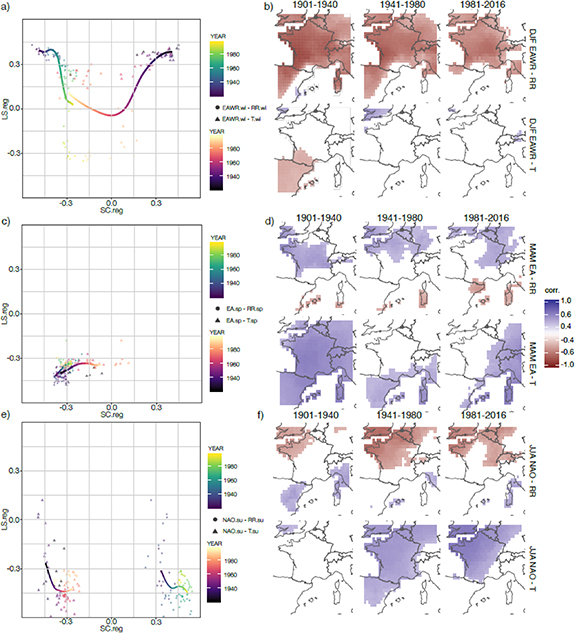
Figure 5. (a) Scatterplot between obtained standardized regression coefficients using winter EAWR (y-axis) and winter surface climate (x-axis, RR—precipitation and T—temperature) as predictors for total soft wheat yield aggregated at national level. The color gradient in points represents the central year of the 40-year period used to obtain the regression coefficient. (b) Correlation between surface precipitation (and temperature) anomalies and EAWR during winter in three successive periods. (c) Same as a), but for EA indicator and surface climate in spring. (d) Correlation between surface precipitation (and temperature) anomalies and EA during spring in three successive periods. (e) Same as (a) but for grain maize and NAO in summer. (f) Correlation between surface precipitation (and temperature) anomalies and NAO during summer in the three successive periods.
Download figure:
Standard image High-resolution imageThe second prominent pattern, the spring EA, relates to positive precipitation anomalies in the central-northern part of France (figure 5(c)), is characterized by more stable and lower temporal variation of regression coefficients through time. As for the surface temperature, the strong positive correlation observed at the beginning of the 20th Century disappeared later on and only remained significant in the southern and eastern parts of France. Consequently, the share of wheat area affected by this pattern decreased after the 1940s, followed by an increase towards the end of the analysis period. Comparison with the impact of surface climate variables suggests that EA imposes a stronger control on precipitation anomalies when it comes to impact on wheat yield; indeed, towards the end of the analysis period the regression coefficient remains significant for the EA spring pattern, however the surface temperature impact diminishes (figure 2).
As shown in figures 2 and 3, the LS circulation impact on inter-annual crop yield variations exhibits a time-varying behaviour in terms of strength of impact as well as the share of cropland area affected. Temporal variation in regression coefficients can arise from different sources: (i) changing sensitivity of crop yields to climate anomalies, which originates from agro-management practices such as changing crop varieties and introduction/improvement of various agro-management practices (e.g. irrigation; Van der Velde et al 2010, Ceglar et al 2016), (ii) changes in covariance between LS indexes, and (iii) time-varying LS circulation impact on regional surface climate. The latter is likely to change the relation between the LS circulation and its regional climate impact. These variations are related to changes in the mean state of the climate system over which the circulation anomalies are over-imposed, such as sea surface temperature, sea ice, or snow cover over land. Temporal variation of LS circulation impact in the northern Atlantic region can be related to displacement of NAO's action centres and consequently changed atmospheric flow (Schenk et al 2009).
Time-varying behaviour of established regression models can be observed also in the temporal evolution of explained variability (figures 4(a) and (c)). The amount of variability explained by LS circulation decreases consistently for all types of wheat towards the mid-of Century and increases again in the 1970s. By contrast, the amount of variability explained by surface climate is steadily decreasing until it reaches a stable value of nearly 40% after the 1970s. It is interesting to observe that LS circulation explains more variability than surface climate after this point in time. There are several possible reasons for this. Surface climate based regression models take into account only precipitation and temperature; other variables could play an important role for instance when it comes to the prevalence of diseases. Additionally, isolated extreme events during the most sensitive growth stages are not captured properly due to the seasonal aggregation (e.g. Porter and Semenov 2005). On the other hand, the LS circulation control over surface climate also affects other weather characteristics, such as wind speed, humidity, and solar radiation. At the same time, however, derived relationships using LS patterns are complicated by the nonstationarities induced by other factors such as sea surface temperatures and Quasi-Biennial Oscillation (related to stratospheric warming and cooling events), that are difficult to isolate and control in our regression models. For example, when the Atlantic is cold, the NAO tends to be more often in a positive state; when the Atlantic is warm, the situation is reversed (D'Aleo and Easterbrook 2016). The weaker control of large-scale circulation over wheat yields during the mid-century period warrants additional research on modulation of LS circulation in the northern Atlantic region due to Atlantic Multidecadal Oscillation (Zhang et al 2019), as the impact of the latter on western European climate is especially strong in spring (Zampieri et al 2017b).
It is worthwhile mentioning that regional surface climate always explains a higher proportion of observed maize yield variability than the LS patterns (figure 4(c)). During the summer, the impact of LS circulation on surface climate (especially rainfall) becomes weaker, as surface processes become relevant (e.g. increased convection activity). Nevertheless, a positive summer NAO phase, which favours warm temperature anomalies in France, has increased its influence on maize areas in France (figure 6(b)).
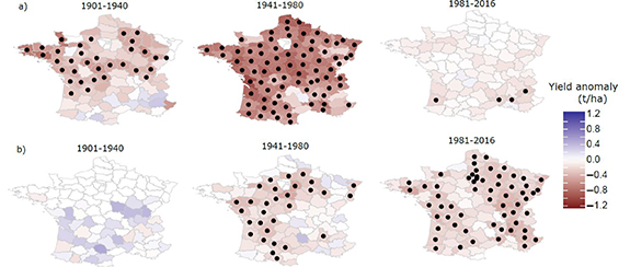
Figure 6. (a) Difference in observed total soft wheat yield anomaly in crop growing seasons when a compound event occurred characterized by a negative winter EAWR and a positive spring EA, and all other growing seasons, for three time periods. Black dots denote whether the difference is statistically significant (p < 0.05). (b) Difference in observed grain maize yield anomaly in crop growing seasons when summer NAO was positive and growing seasons with negative summer NAO.
Download figure:
Standard image High-resolution image
Figures 4(a) and (c) reveals another important feature; the evolution of explained yield variability for both crops is more stable when surface climate is used to provide explanatory variables. This has important implications for prediction purposes. In terms of statistically modelling the impact of surface climate change on crop yield anomalies, regression models can be estimated more reliably when using surface climate as predictors for at least a decadal window ahead of the calibration period, assuming that agro-management effects (important for estimation of crop yield trends) are known or can be extrapolated from trend analysis. For example, given the relatively stable persistence of summer temperature and precipitation regression coefficients for grain maize in the 1950s, these models could be used to estimate the effects of summer climate impact almost until the end of our analysis period. In the case of wheat, the decadal predictability seems weaker mainly due to the longer growing season and thus an interplay of many more different variables compared to grain maize. The LS based empirical models can still be used to forecast the yield one to several years ahead of the training period. This has important implications for using seasonal forecasts of LS circulation patterns, which are generally more skilful than seasonal surface climate forecasts (e.g. Stockdale et al 2015, Dunstone et al 2016).
4.3. Case study—diverse impact of LS on crop yields in two distant periods
To further illustrate the high level of time-varying LS impact on regional crop yields, let us consider several years with observed wheat yield anomalies under the lower tercile values. According to estimated regression coefficients, the compound events with negative winter EAWR (positive precipitation anomalies) and positive spring EA (warm and wet spring) provide highly unfavourable conditions for wheat yields. Such a year occurred in 1947 (figure 1(a)), which resulted in the lowest standardized wheat yield anomaly during the last century. Strong blocking persisted over north-western Europe during the second half of January which favoured an inflow of cold air from north-eastern Europe and diverted the westerly flow of Atlantic depressions towards the south of Europe. France experienced extreme cold weather in the north and mild temperatures with excessive wetness in the south and south-western parts (Eden 2008). The winter crops in the north were therefore exposed to frost kill (FAO 1947). The winter was followed by a wet spring, further compromising crops that survived the preceding winter frost. Even though the extremity of this compound event was unique in the entire period after 1901, its occurrence in other growing seasons before the 1980s resulted in significantly lower yields with respect to other years (figure 6(a)). However, the occurrence of these compound events after the 1980s did not result in significantly different yields than in other years, except in a couple of regions in southern France. The different nature of winter climatic extremes occurring in the north and south of France in 1947 also demonstrate the importance of regional assessments on crop yield impact.
France experienced one of the worst soft wheat yield losses in 2016 (in terms of detrended crop yield anomalies, figure 1(b)). This loss was a consequence of a compound event consisting of abnormally warm temperatures in late autumn/early winter and abnormally wet conditions in the following spring (Ben-Ari et al 2018). In terms of LS circulation patterns, these climate conditions are favoured by strong positive EA patterns during autumn, winter and spring; and warm winter is favoured also by a positive NAO. While both empirical models (trained on LS patterns and surface climate) result in a slightly negative yield anomaly on national level for that year, they both fail to capture the magnitude of the 2016 yield loss in France. A relatively small area was affected by large scale circulation; figure 2(a) shows that roughly half of the wheat area is affected by the spring EA pattern and only one quarter of area is affected by autumn EA. Additionally, a stronger signal from large-scale circulation is hidden in the seasonal values, which represent an average over three months. Excessive wetness in May 2016 is only partially captured by the EA signal; a better explanatory variable in this case could be the SCAND pattern for May, which was highly positive (i.e. favouring positive precipitation anomalies over France). Indeed, this situation was caused by an almost stationary low pressure system over France and Germany, leading to heavy rainfalls in different locations (Oldenborgh et al 2016). Similarly, the EA pattern in preceding December 2015 was extremely high, favouring abnormally warm temperatures. These probably contributed to increased disease pressure, indirectly influencing the final wheat yields (Ben-Ari et al 2018).
5. Conclusions
We have derived a statistical framework to identify the temporal stability of large scale circulation impact on French crop yields using reported regional crop yields since the beginning of the 20th Century. A lack of temporally consistent impact on crop yields for both main crops (soft wheat and grain maize) grown in France is identified. The winter EAWR had a dominant impact on soft wheat yields until the 1980s; additionally, yield became sensitive to large scale climate forcing in autumn during the second half of the 20th Century (SCAND and EA patterns), while the sensitivity to winter circulation features gradually weakened towards the last third of the analysed period. By contrast, the LS patterns in spring (EA and SCAND patterns) have increased their influence during the last third of the analysis period (1981–2016). Grain maize has been mainly affected by summer SCAND and NAO patterns, with the former having a higher influence at the beginning, and the latter towards the end of the 20th Century. Both patterns can be linked to the deteriorating impact of positive temperature anomalies and negative precipitation anomalies on maize yields.
The amount of crop yield variability explained by LS circulation decreases for soft wheat towards the mid of the 20th Century and increases again in the 1970s. Conversely, the amount of variability explained by surface climate is steadily decreasing until it reaches a stable value in the 1970s. The fact that surface climate, expressed in terms of seasonal average temperature and precipitation cumulates, explains less variation in wheat yield anomalies as LS patterns do, reveals the importance of extreme surface climate events such as precipitation shortages and heat stress during more sensitive growing periods. Surface climate consistently explained a higher share of crop yield variance than the LS patterns counterpart throughout the entire period for grain maize. Our analysis also reveals temporally varying crop area totals affected significantly by climate conditions. This highlights the importance of regional impact assessments of both LS patterns and surface climate on crop yields.
The LS patterns have an important impact on soft wheat and grain maize yields in France, albeit with high levels of temporal variation. This limits the use of derived empirical models for prediction of yield anomalies beyond a seasonal time scale in a decadal to multi-decadal setting (e.g. simulation of future climate change impacts). Two main reasons behind this are the non-stationary large scale control over surface climate and changes in agricultural practices (such as introducing new varieties, irrigation and fertilization); their combined effect can lead to different levels of sensitivity of crops to climate anomalies, when distant periods are considered. Nevertheless, we have identified a source of seasonal predictability (i.e. up to one year ahead) for soft wheat and grain maize crop yields. This framework could take advantage of potentially higher skill of seasonal predictions of large-scale atmospheric circulation as opposed to surface climate in mid-latitudes. It is important, though, to constantly re-calibrate the empirical models using the most recent crop yield observations.
Acknowledgments
The authors would like to acknowledge support from H2020 MedGOLD project (grant No. 776467).
Data availability
The data that support the findings of this study are available from the corresponding author upon reasonable request.