

Abstract
Seasonal mean atmospheric circulation in Europe can vary substantially from year to year. This diversity of conditions impacts many socioeconomic sectors. Teleconnection indices can be used to characterize this seasonal variability, while seasonal forecasts of those indices offer the opportunity to take adaptation actions a few months in advance. For instance, the North Atlantic Oscillation has proven useful as a proxy for atmospheric effects in several sectors, and dynamical forecasts of its evolution in winter have been shown skillful. However the NAO only characterizes part of this seasonal circulation anomalies, and other teleconnections such as the East Atlantic, the East Atlantic Western Russia or the Scandinavian Pattern also play an important role in shaping atmospheric conditions in the continent throughout the year. This paper explores the quality of seasonal forecasts of these four teleconnection indices for the four seasons of the year, derived from five different seasonal prediction systems. We find that several teleconnection indices can be skillfully predicted in advance in winter, spring and summer. We also show that there is no single prediction system that performs better than the others for all seasons and teleconnections, and that a multi-system approach produces results that are as good as the best of the systems.
Export citation and abstract BibTeX RIS

Original content from this work may be used under the terms of the Creative Commons Attribution 4.0 license. Any further distribution of this work must maintain attribution to the author(s) and the title of the work, journal citation and DOI.
1. Introduction
Atmospheric circulation in Europe and the North Atlantic has a strong seasonal cycle, but it can also vary substantially from one year to another in the same season. The year-to-year climate variability can partly be attributed to the chaotic nature of the atmosphere but also to external forcings exerted by other components of the Earth system such as ocean temperature, soil moisture or sea ice extent anomalies that modify the energy budget of the atmosphere and ultimately modify the large-scale circulation (Doblas-Reyes et al 2013, Heinze et al 2019, Mariotti et al 2018). This interannual variability has strong impacts on several socioeconomic sectors such as energy, agriculture, tourism, insurance, water management, health or civil protection among others (Hewitt et al 2012, WMO 2014). Therefore seasonal forecasts that provide climate information for the next few months are very useful to take precautionary actions and adapt to anomalous climate conditions in advance (Soares et al 2018, White et al 2017, Torralba et al 2017, Ceglar et al 2018, Walz et al 2018, Turco et al 2018, Clark et al 2017).
Seasonal climate variability over Europe is often analyzed through atmospheric teleconnections. The rationale behind atmospheric teleconnections is to find recurrent and persistent large-scale atmospheric circulation patterns and corresponding temporally varying indices that can be used to describe monthly or seasonal climate variability and its surface impacts in a simplified way. For instance, the North Atlantic Oscillation (NAO) (Hurrell et al 2003, Wanner et al 2001), the most relevant Euro-Atlantic teleconnection, is known to affect surface temperature, precipitation and wind speed in almost all of Europe (Trigo et al 2002, Brayshaw et al 2011). However the NAO only represents around one third of the seasonal circulation variability over Europe in winter, spring and summer (in autumn represents only one sixth), while other Euro-Atlantic Teleconnections (EATC) such as the East Atlantic (EA) (Woollings et al 2010), the East Atlantic/Western Russia (EAWR) (Lim 2014) and the Scandinavian pattern (SCA) (Bueh and Nakamura 2007) also play an important role in modulating surface conditions (see for example Zubiate et al (2016), Josey et al (2011) or Hall and Hanna (2018)).
Several authors have recently shown that the state of the NAO during winter (DJF) can be skillfully predicted months or even more than a year ahead employing dynamical prediction systems that simulate the interactions between atmosphere, ocean, sea ice and soil moisture conditions (Scaife et al 2014, Smith et al 2014, Dunstone et al 2016, Johnson et al 2019). The use of multi-system prediction ensembles can achieve even better results (Athanasiadis et al 2017, Baker et al 2018). However, the ability of state-of-the-art seasonal forecast systems to simulate the other EATC indices has not yet been systematically explored in the literature. Only empirical predictions of the EA index derived from sea surface temperature in the preceding months have been proved useful in summer (Ossó et al 2017, Iglesias et al 2014), while a point-based sea level pressure index that resembles the EA has been studied for winter in Baker et al (2017). Therefore it would be highly beneficial to produce and analyse dynamical forecasts for the other EATC indices (Hall and Hanna 2018). Also, the focus of most of the previous studies has been on the winter season, while forecasts for the other seasons can be relevant as well for many seasonal climate service users. Therefore a systematic approach that can be employed throughout the year for all the EATCs and for both observations and seasonal prediction systems has been defined in this work.
Teleconnection patterns and indices can be computed in many different ways. Essentially, point-based, box-based or Empirical Orthogonal Function analysis methods are used in the literature. A typical method to define those teleconnections is through Rotated Empirical Orthogonal Function (REOF) analysis (Barnston and Livezey 1987). REOF is a dimensionality reduction technique that allows for approximating circulation anomalies as a linear combination of only a few spatial patterns:
Teleconnection Patterns (TCP) and Indices (TCI) –i.e. the weights in the linear combination—are chosen so that the residual term is minimized. Over the Euro-Atlantic region, when retaining four variability modes the aforementioned teleconnections (NAO, EA, EAWR and SCA) are obtained. This methodology mimics well-known Climate Prediction Center patterns and indices as much as possible (Climate Prediction Center 2012), and does not rely on identifying the centers of action of the different teleconnections, which move from one season to another. Additionally, point-based indices are sensitive to model biases and local skill at the centers of action. Indeed Athanasiadis et al (2017) have already shown that the highest skills for NAO forecasts are obtained when using spatially-averaged indices.
The observed patterns and indices for these four Euro-Atlantic Teleconnections (EATC) have been obtained from ERA5 reanalysis, and forecasts of each EATC index have been derived from multiple seasonal prediction systems by projecting predicted circulation anomalies onto the observed teleconnection patterns. Employing this method, the skill of several seasonal prediction systems from the Copernicus Climate Change Service (C3S) in simulating the year-to-year variability of the NAO, EA, EAWR and SCA teleconnection indices for the four seasons of the year, and from zero to three months before the start of the season has been analysed. Section 2 describes the data and methods employed in detail, section 3 presents the results and conclusions follow in section 4.
2. Datasets and methodology
2.1. Datasets
2.1.1. Observational reference
The ERA5 reanalysis (Copernicus Climate Change Service 2019, Copernicus Climate Change Service (C3S) 2017) from the European Center for Medium-Range Weather Forecasts (ECMWF) has been employed as observational reference to define the four Euro-Atlantic teleconnection patterns and indices for the 1981–2018 period. More specifically, seasonal anomalies of geopotential height at 500 hPa with respect to the whole period have been obtained separately for each of the four seasons (DJF, MAM, JJA and SON). Although the ERA5 data has a spatial resolution of ∼0.28 degrees (or ∼30 km), in order to obtain teleconnection patterns that can be compared with the seasonal prediction systems, the data has been regrided to match the spatial resolution of the forecasts (1 x 1°, see table 1).
Table 1. Summary of the seasonal prediction systems employed.
| Producing center | Prediction system | Data source | Analyzed period | Ensemble members | Ensemble generation | Horizontal grid |
|---|---|---|---|---|---|---|
| CMCC | SPS3 | CDS | 1993-2016 | 40 | burst | Regular 360x180 |
| DWD | System2 | CDS | 1993-2016 | 30 | burst | Regular 360x180 |
| UKMO | GloSea5 GC2 | CDS | 1993-2016 | 28 | lagged | Regular 360x180 |
| MF | System6 | CDS | 1993-2016 | 25 | lagged | Regular 360x180 |
| ECMWF | SEAS5 | CDS | 1993-2016 | 25 | burst | Regular 360x180 |
| ECMWF | SEAS5 | MARS | 1981-2016 | 51 | burst | Regular Gaussian F160 (640x320) |
2.1.2. Seasonal prediction systems
Several European national meteorological centers and institutions produce operational seasonal predictions. Those are made with coupled Earth system models that simulate the evolution of atmosphere, ocean, sea ice and land surface conditions in the upcoming months. Five different seasonal prediction systems have been employed in this study, from the European Centre for Medium-Range Weather Forecasts (ECMWF), Deutscher Wetterdienst (DWD), Météo France (MF), UK Met Office (UKMO) and Centro Euro-Mediterraneo sui Cambiamenti Climatici (CMCC). The latest operational prediction systems (at the time of writing) from those centers have been employed: SEAS5 from ECMWF (Johnson et al 2019), Seasonal Prediction System 3 from CMCC (SPS3) (Sanna et al 2017), System6 from MF (MF6) (Dorel et al 2017), GloSea5-GC2 from UKMO (GS5GC2) (MacLachlan et al 2014, Williams et al 2015) and System2 from DWD (DWD2) (Deutscher Wetterdienst 2019). All of the predictions have been obtained from the Climate Data Store (CDS) of the Copernicus Climate Change Service (C3S) initiative, which provides a unified access point, and a common hindcast period and spatial resolution (ECMWF 2019). The most relevant details of each one of the prediction systems employed here, such as the number of ensemble members, the hindcast period analyzed or the spatial grid are specified in table 1. Notice that the ECMWF SEAS5 predictions have been additionally obtained for a longer period and bigger ensemble from ECMWF MARS service, and used in section 3.3 to test the sensitivity of the results to the period length and the ensemble size.
The configuration of those prediction systems is similar in terms of initialization, numerical integration, parametrizations and coupling of the different Earth system components modelled. However GS5GC2 and MF6 have a lagged ensemble—produced by accumulating several integrations initialized at different instants of time during the latest month—while the other systems are initialized in burst mode the first day of the month—perturbed initial conditions and stochastic parametrizations are used to initialize and run several ensemble members in order to describe uncertainty—. The MF6 hindcast ensemble is built from 1 ensemble member initialized the first of the month plus 12 members initialized the 25th of the previous month and 12 members initialized the 20th of the previous month. Similarly, the GS5GC2 hindcast ensembles are built from 7 members initialized the first of the month, plus 7 members for the 9th, 17th and 25th of the previous month respectively (see ECMWF (2019)). The hindcast for GS5GC2 has been built by combining two versions of this system: all the System13 hindcasts available in the CDS with a few System14 runs for May to October 2016.
The 500 hPa geopotential height fields of these systems were downloaded, formatted and quality checked with an in-house developed python software suite that automatically processes the data to a common format (NetCDF). Quality controls include file integrity, time and ensemble members completeness and consistency, missing values, and physical value checks. These checks detected issues in 28 fields of 500 hPa geopotential height of the SPS3, distributed across all the period and ensemble. The issues were reported to C3S and confirmed by the data provider, and have been documented under known issue E5a in the C3S portal (https://confluence.ecmwf.int/ display/ CKB/ C3S+ Seasonal+Forecasts+known+issues). The affected members and months have been not included in the analysis. Given the relatively low number of erroneous fields (28 out of 80 640), this should not produce noticeable effects on the results. However keeping the erroneous fields would produce a significant skill degradation.
2.2. Methods
2.2.1. Observed teleconnection patterns and indices
The four observed EATC patterns and indices have been computed from ERA5 500 hPa geopotential height seasonal anomalies through a Rotated Empirical Orthogonal Function (REOF) analysis (Hannachi et al 2007, Wilks 2019) over the Euro-Atlantic domain (90°W–60°E and 20°N–80°N). First, seasonal anomalies for each season (DJF/MAM/JJA/SON) and for the 1981–2018 period have been computed with respect to the same period mean. Then an EOF analysis has been performed, and the first four variability modes have been retained. The anomalies have been weighted by the cosine of the latitude prior to the EOF analysis to account for differences in the areas of the grid points. After that, a Varimax rotation has been applied to the unit length eigenvectors (or loading patterns), in order to simplify the spatial structure of the patterns but still preserve its orthogonality (Mestas-Nuñez 2000). Finally, the four obtained REOF modes have been reordered and their sign has been adjusted when needed so that the EATC patterns resemble as much as possible the positive phases of the NAO, EA, EAWR and SCA patterns as computed by NCEP's Climate Prediction Center (Climate Prediction Center 2012, Barnston and Livezey 1987, Lim 2014). Figure 1 shows the four teleconnection patterns (i.e. the rotated unit-vector loadings after readjusting for the latitudinal weights) obtained for each of the four seasons of the year. Due to the normalization, the more localized patterns such as the EA have strongest colors in the figure, while more widespread patterns such as the NAO have lighter colors. The percentage of variance that each of the EATC patterns represents can be seen in figure 3 lower left panel for each season. While NAO represents around one third of the total variance in winter, spring and summer, the other EATC patterns also contribute to describe the atmospheric circulation variability with values of up to 20% of explained variance. The residual variance that remains unexplained by the four EATCs in each season (i.e. the variance of the residual term in equation (1)) indicates the goodness of the approximation of the circulation anomalies by the four EATCs, and expressed as a percentage of the total variance it is: 23% (DJF), 36% (MAM), 33% (JJA) and 36% (SON). This is much less than when only using the first EOF to compute the NAO (always above 60%).
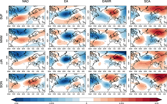
Figure 1. The loading patterns (i.e. of norm one) of the four Euro-Atlantic teleconnections obtained for each season from ERA5 geopotential height anomalies at 500 hPa in the 1981–2018 period.
Download figure:
Standard image High-resolution image2.2.2. Forecasts of EATC indices
To obtain retrospective forecasts of the EATC indices, the 500 hPa geopotential height fields from the seasonal prediction system hindcasts initialized in the 1993–2016 period have been used (note that the ERA5 EATCs have been computed with a longer period to obtain more robust patterns). The seasonal mean anomalies of each system (with respect to its own climatology in the 1993–2016 period) and for each season have been projected onto the observed patterns, individually for each ensemble member. To do so, first the anomalies are weighted by the cosine of the latitude, and then the scalar product with each teleconnection pattern is computed. The projected indices have not been normalized, so that the explained variances can be computed by just doing the scalar product of each projected EATC index by itself. The total variance of each prediction system has also been computed and normalized per number of grid points, years and ensemble members, so that results can be compared with observed variance.
2.2.3. Multi-system ensemble predictions
Combining the information from several prediction systems into a single forecast can be beneficial for the forecast quality. Each prediction system represents physical processes in slightly different ways. Hence, it has been shown that the combination of all the ensemble members from different systems tends to compensate modelling errors and uncertainties from different sources (DelSole et al 2014). The larger ensemble size of the combination also contributes to cancel noise in the individual members and extract smaller forcing signals (Scaife et al 2014, Baker et al 2018). Two multi-system combinations have been produced here (as in Doblas-Reyes et al (2003) and Athanasiadis et al (2017)): first by pooling all the ensemble members together (MSPool) and secondly by weighting each prediction system by combining the ensemble means computed separately in each system so that all systems have equal weight in the final results (MSEW).
2.2.4. Forecast quality assessment
The quality of the EATC forecasts has been assessed employing both deterministic and probabilistic skill metrics. First the ensemble mean correlation has been used as a measure of association. The statistical significance of ensemble mean correlations has been checked with a one-tailed Student's t-test at a level of 95% of confidence. Additionally, the Ranked Probability Skill Score (RPSS) has been employed (as in Doblas-Reyes et al (2003) for NAO forecasts) to understand the improvement of tercile forecasts of EATC indices over a climatological benchmark (Jolliffe and Stephenson 2011). This score assesses the quality of a probabilistic forecast that delivers probabilities of having a below normal, normal or above normal value of an EATC index. Those categories are defined based on the 33rd and 66th percentiles (i.e. terciles) of the historical distribution of forecast values in the hindcast. The uncertainty affecting the RPSS values has been explored in terms of the Diebold-Mariano test (Diebold and Mariano 1995). This test allows to identify if the differences between a probabilistic forecast and the climatological forecast (the reference here) are statistically significant at the 95% confidence level. The Diebold-Mariano test from the SpecsVerification R package has been employed.
The assessment has been performed for all seasons, and employing the forecasts initialized at the beginning of the season and also from 1 up to 3 months before. The elapsed time between the initialization date and the start of the valid period of the forecasts is the lead time, which has been referred to as lead 0, 1, 2 and 3 to indicate the number of months of lead time. For lagged ensembles, the latest initialization date in the ensemble is employed to compute the lead (i.e. lead times are counted since the first day of the month, when all the ensembles are built). All the verifications correspond to the start dates in the 1993–2016 period. Table 2 summarizes the start dates and valid date periods employed for each season. Notice that DJF forecasts initialized in the 1993–2016 period correspond to 1993/94 to 2016/17 winters. The MAM season requires special attention: since predictions initialized in December 1992 are not available in the CDS, the 1993 start dates for January, February and March (JFM) were also discarded in order to obtain consistent results across all lead times. Therefore the verification of forecasts for spring has one year less than the other seasons. This fine-detail information is essential for reproducibility in view of the sensitivity of results to the hindcast period employed (see section 3.3).
Table 2. Summary of the forecast start months employed for verification in each season and the corresponding valid periods.
| Valid period | Forecast start dates |
|---|---|
| JJA 1993–2016 | MAMJ 1993–2016 |
| SON 1993–2016 | JJAS 1993–2016 |
| DJF 1993/94–2016/17 | SOND 1993–2016 |
| MAM 1994–2016 | D 1993–2015 |
| JFM 1994–2016 |
The focus of the verification is on assessing the quality of the products as available to end users. Therefore, no correction has been applied to compensate for the differing number of ensemble members across systems, nor for the longer lead times of the older members in lagged systems.
3. Results
To illustrate how the seasonal prediction systems simulate the ERA5 EATC indices, figure 2 shows the seasonal predictions of the four EATC indices issued in November and valid for DJF (i.e. 1 month of lead time) for each of the systems in the 2000 1993–2016 period. All the systems agree in a negative NAO phase for 2009/2010 winter (first panel), although the actual observed value was well below the range of any prediction. Less well-known events such as a strong EA phase in 2013/2014 or a strong SCA phase in 2009/2010 can also be seen. As the forecasted teleconnection indices have not been normalized, a widest range can be seen for the NAO than for the other three EATCs.
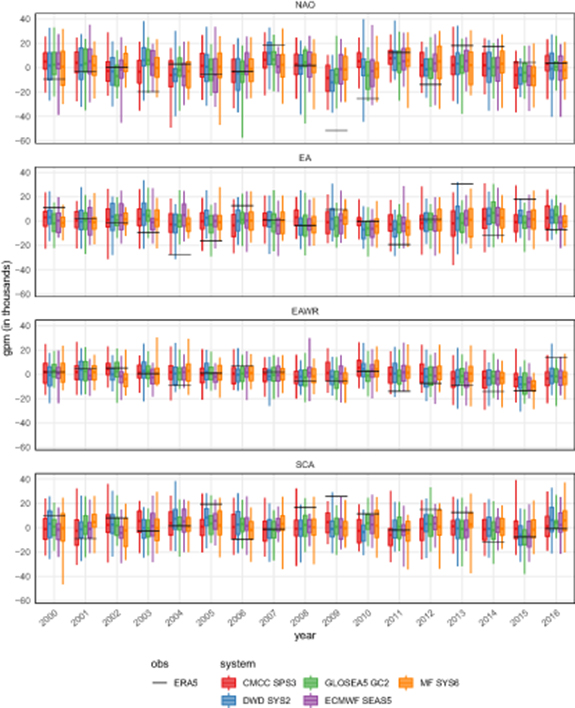
Figure 2. Retrospective forecasts of the four EATC indices issued in November and valid for DJF (i.e. one month of lead time) for each of the prediction systems in the 2000–2016 period. Each boxplot shows the maximum and minimum forecast value (whiskers), the first and third quartiles (box) and the ensemble mean (color line). The black line denotes the observed value according to ERA5. The year labels correspond to the forecast start date (i.e. November). The vertical axe represents geopotential meters, so that when those non-normalized EATC indices are multiplied by the loadings, an approximation of the original anomalies is obtained.
Download figure:
Standard image High-resolution image3.1. Variance explained by each EATC in the prediction systems
In order to understand how well the observed teleconnection patterns describe the variability in each of the prediction systems, the explained variance of each EATC pattern as a percentage of the total variance in the system has been analysed for the 1993–2016 period. The explained variance percentages have also been computed for ERA5 in the same period. The differences between explained variance percentages in the prediction systems and in ERA5 is displayed in figure 3 for each season, lead time and EATC pattern. Additional analyses revealed that those differences are not due to sampling variability (not shown). In general, all prediction systems have less proportion of NAO variability than observed in winter, spring, and specially in summer. Something similar occurs with the EAWR pattern in autumn or the EA in winter. On the other hand the NAO has slightly more variability than observed in most prediction systems in autumn and the same occurs for the EAWR in winter and the EA in spring. Most of these differences in variability show up already from lead 0 forecasts, and do not grow with higher lead times, indicating a small role of model drift. In terms of absolute variance, all of the systems have a good agreement with the ERA5 variance (not shown), i.e. the total amount of variability in the prediction systems is comparable to that in the observational reference for the four seasons.

Figure 3. Biases in the percentage of the total variance explained by each EATC for each prediction system, lead time and season with respect to the explained variance in ERA5 (bottom-left panel) for the same period (1993–2016).
Download figure:
Standard image High-resolution imageThese biases show that variability has a different structure in the prediction systems than in the observations. This might be related to the internal variability modes of the prediction systems do not match the observed ones, i.e. there are biases in location and shape of the EATC patterns directly obtained from the prediction systems (e.g. see Walz et al (2018) for a comparison of the internal variability modes of a seasonal prediction system and a reanalysis in winter).
3.2. Forecast quality of EATC predictions
The ensemble mean correlation has been widely used to verify ensemble predictions of the NAO. The process of averaging the teleconnection index predictions from several individual members produces the effect of cancelling the noise present in each single realization and allows extracting any forcing signal that is common to the different members. Figure 4 summarizes the ensemble mean correlation results for all systems, seasons, lead-times and teleconnections in a graphical way. A first sight reveals important differences between seasons, while there is a good degree of agreement between different prediction systems on which teleconnections have a positive and statistically significant correlation. In winter (top left) all systems show positive correlations for the NAO and SCA at the start of the season, while SEAS5 and MF6 systems still show significant correlations in the forecasts issued in September (lead 3). The EA also has positive and significant correlations for some systems at lead 0. In spring (top right) and at lead 0, all the teleconnections have positive correlations in almost all of the systems. However, at longer lead times the correlation values become weaker and statistically non-significant. In summer (bottom left) the NAO and SCA indices show very good correlation levels for all lead times and almost all systems. The EA and EAWR correlations are only statistically significant at lead 0 for SEAS5 and DWD2 respectively. Autumn shows the worst results overall. The EA shows statistically significant correlations only in lead 0 but for almost all systems. Surprisingly, the SCA shows also positive and significant correlation levels at lead 3 for SPS3, SEAS5 and MF6 systems, but not for any other smaller lead time.
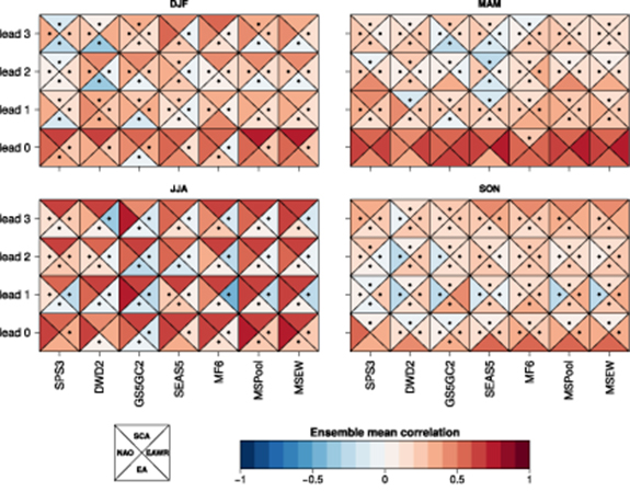
Figure 4. Correlation between the ensemble mean of the EATC forecasts and the corresponding observed (ERA5) values for each system, lead time and season in the 1993–2016 hindcast period. Black dots indicate cases were the correlation is not found statistically significant at the 95% of confidence level.
Download figure:
Standard image High-resolution imageMost of the non-significant correlations are still positive. This might be a sign that although small, those correlations are not just random outcomes (which should be distributed evenly into positive and negative values), but rather that the signal-to-noise ratio is too low in those cases for the significance test to be able to detect it. This is consistent with some works that have shown the difficulties to provide skillful seasonal climate predictions in the Euro-Atlantic region as a consequence of the excessive role that internal variability plays in prediction systems in that region (Scaife and Smith 2018). This issue has been further explored in the following section.
The results for winter NAO predictions are in line with previous published research (Scaife et al 2014, Baker et al 2018, Athanasiadis et al 2017, Johnson et al 2019), taking into account the different methodologies employed and also the high variability of verification metrics due to the verification period employed (see section 3.3 below).
Multi-system predictions that combine the members from several prediction systems (MSPool and MSEW; see section 2.2.3) tend to perform very good in terms of ensemble mean correlation. This is partly due to an increase of the ensemble size by around five times compared to the individual systems, but also thanks to the cancelling of modelling errors from different systems. Although many times there is a single model that does better for a given teleconnection index, overall the multi-system shows more stable results through the lead-times and indices and is always very close or above the best system. The two multi-system methods produced almost identical performance. For that reason and for simplicity, the RPSS has been only computed for the MSPool method.
The RPSS corresponding to the EATC indices for all seasons, lead-times, and systems has been plotted similarly in figure 5. The plot shows very similar results to the ensemble mean correlations, in general terms, although the absolute values of RPSS are much lower than those of correlation. Some differences in terms of statistical significance of the results can be seen. For example, figure 5 (bottom-left) shows that the NAO RPSS in JJA is not significant in SEAS5 and MF6 beyond lead 0, however, correlation values were statistically significant in all the lead times and seasons (figure 4). On the other hand, RPSS for the EA index in DJF (lead 0) in the MF6 system is significant while correlation is not.

Figure 5. Ranked probability skill score of EATC tercile forecasts for each system, lead time and season in the 1993–2016 hindcast period. Black dots indicate cases were the RPSS is not found statistically significant at the 95% of confidence level.
Download figure:
Standard image High-resolution imageBoth employed metrics analyze different aspects of the predictions and therefore cannot be numerically compared. The RPSS is in general a more restrictive quality measure than ensemble mean correlation. For instance, Kumar (2009) showed that randomly-generated forecasts with similar levels of signal-to-noise ratio reach higher ensemble mean correlations than RPSS values. Also, ensemble calibration techniques such as variance inflation (Doblas-Reyes et al 2005, Torralba et al 2017) could be employed to adjust the EATC forecasts and obtain more reliable predictions. This would translate in better RPSS values, although the ensemble mean correlation would not change. These considerations show that it is necessary to consider more than one metric to derive meaningful conclusions.
3.3. Sensitivity of ensemble mean correlation to hindcast period and number of members
Previous research has found that ensemble mean correlation of NAO is sensitive to hindcast length and ensemble size (Baker et al 2018, Siegert et al 2016, Kumar 2009). To further verify this for the other EATCs, the ECMWF SEAS5 hindcast from MARS have been employed. This hindcast has a longer period (1981–2018) than the C3S hindcast, and for the November initialization it has 51 ensemble members. By subsetting the number of years and the number of members included in the verification, we can evaluate the sensitivity of the correlation and RPSS results to the ensemble size and the hindcast length. For each EATC index, a collection of 10 000 random subsets of 25 members out of the 51 available are used to draw a distribution of verification results. In the same way, a collection of 10 000 subsets of 25 years out of the 38 available is used to produce one distribution of verification values for each EATC. Figure 6 shows the results in violin plots (which enhance typical boxplots with information from the whole distribution). The variability is very large both for correlations (top panels) and for RPSS (bottom panels), with ranges of values of more than 0.5 points in correlation, and 0.2 points in RPSS. The spread of the distributions is very similar among different EATCs, indicating that this uncertainty is not intrinsically related to NAO variability but is a general issue of seasonal predictability over Europe. The variability when subsetting the period (right panels) is a bit larger than the variability when subsetting the members (left panels), for all the EATCs. The mean value of the distributions (not shown) is slightly higher when the period is subsetted. The effect of adding more years is to get a more reliable estimate of skill, but adding more members will tend to produce higher skill scores due to a higher cancellation of noise in bigger ensembles. From this analysis it is clear that the verification of both deterministic and probabilistic EATC forecasts requires large ensembles and large hindcast periods. As a consequence, all the results presented in previous sections, although very useful to characterize the EATC prediction skill in the current operational seasonal prediction systems, have to be cautiously interpreted.

Figure 6. Sensitivity of ensemble mean correlation and RPSS for each EATC to the hindcast years and the number of ensemble members included in the verification. The SEAS5 hindcast for MARS (covering 1981–2018 with 51 members) has been subsetted 10 000 times to produce a distribution of values.
Download figure:
Standard image High-resolution image
4. Conclusions
A method to produce seasonal forecasts of NAO, EA, EAWR and SCA indices for the four seasons and from five different seasonal prediction systems available in the C3S CDS has been developed. Retrospective predictions of those indices for the 1993–2016 period have been verified. A few conclusions can be drawn from the results:
- Prediction skill is not limited to NAO: atmospheric variability shaped like EA, EAWR and SCA patterns can also be simulated by the seasonal prediction systems.
- Prediction skill is not limited to winter: spring and summer have also similar levels of skill for some teleconnections, while autumn shows only modest scores (probably due to a lower signal-to-noise ratio).
- There is a good degree of agreement between systems in which EATCs can be predicted for each season with different lead times. This might highlight inherent predictability of the teleconnections.
- Multi-system predictions of EATC perform almost as well or sometimes even better than the best system. There is not a single system that produces the best forecasts for all the teleconnections, lead times and seasons. Therefore a multi-system simplifies the application of the method in order to implement an operational climate service.
- Initiatives such as C3S are very helpful to produce such multi-system predictions.
- Both deterministic and probabilistic verification metrics show a strong sensitivity to the ensemble size and hindcast length.
These results open the door to produce an operational climate service that provides forecasts of those teleconnection indices all year round. The forecasts could be used directly as proxies or also be employed to derive forecasts of sectorial indicators or to produce downscaled predictions as in Baker et al (2017).
Acknowledgment
The research leading to these results has received funding from the European Union's Horizon 2020 research and innovation programme under grant agreement n° 776787 (S2S4E).
The authors acknowledge the Copernicus Climate Change Service (C3S) for providing seasonal predictions from several European meteorological centers and the ECMWF for producing the ERA5 reanalysis. All the analyses have been done with R employing the packages s2dverification and SpecsVerification.
Data availability
The data that support the findings of this study are openly available at the Climate Data Store of the Copernicus Climate Change service. The ERA5 data is available at https://doi.org/10.24381/cds.6860a573, and the seasonal predictions can be accessed at https://cds.climate.copernicus.eu.