

Abstract
Climate models predict a strengthening contrast between wet and dry regions in the tropics and subtropics (30 °S–30 °N), and data from the latest model intercomparison project (CMIP6) support this expectation. Rainfall in ascending regions increases, and in descending regions decreases in climate models, reanalyses, and observational data. This strengthening contrast can be captured by tracking the rainfall change each month in the wettest and driest third of the tropics and subtropics combined. Since wet and dry regions are selected individually every month for each model ensemble member, and the observations, this analysis is largely unaffected by biases in location of precipitation features. Blended satellite and in situ data from 1988–2019 support the CMIP6-model-simulated tendency of sharpening contrasts between wet and dry regions, with rainfall in wet regions increasing substantially opposed by a slight decrease in dry regions. We detect the effect of external forcings on tropical and subtropical observed precipitation in wet and dry regions combined, and attribute this change for the first time to anthropogenic and natural forcings separately. Our results show that most of the observed change has been caused by increasing greenhouse gases. Natural forcings also contribute, following the drop in wet-region precipitation after the 1991 eruption of Mount Pinatubo, while anthropogenic aerosol effects show only weak trends in tropic-wide wet and dry regions consistent with flat global aerosol forcing over the analysis period. The observed response to external forcing is significantly larger (p > 0.95) than the multi-model mean simulated response. As expected from climate models, the observed signal strengthens further when focusing on the wet tail of spatial distributions in both models and data.
Export citation and abstract BibTeX RIS

Original content from this work may be used under the terms of the Creative Commons Attribution 4.0 license. Any further distribution of this work must maintain attribution to the author(s) and the title of the work, journal citation and DOI.
1. Introduction
Anthropogenic climate change is expected to change global-scale precipitation patterns, and many of the impacts of climate change are expected to occur through change in mean precipitation, and its extremes, heavy rainfall and drought. Such events have a large effect on society with floods, already one of the most costly natural disasters (Munich Re, 2019), and drought expected to increase in some regions (Collins et al 2013). Both have been linked to impacts including migration (Stapleton et al 2017).
Global mean warming is expected to increase the global moisture content of the atmosphere following the Clausius-Clapeyron relationship (Hegerl et al 2015, Bindoff et al 2013 and references therein). Climate models simulate changes in global mean precipitation of 2%–3% K–1 (Pfahl et al 2017) in response to increases in greenhouse gas concentrations, which is less than the 7% K–1 change in atmospheric moisture expected from the Clausius-Clapeyron equation (Held and Soden 2006, Chadwick et al 2013). This is because atmospheric heating by greenhouse gases and energetic constraints on global precipitation reduce the warming impact on rainfall, compared to that on atmospheric moisture (Stephens and Ellis 2008, Bony et al 2013, Allan et al 2014, Jeevanjee and Romps 2018). Changes in precipitation that are directly linked to warming are reasonably robust between GCMs. In contrast, changes in atmospheric circulation can cause changes in the strength, location and pattern of precipitation features which are far more uncertain and a source of substantial differences in rainfall changes between climate models (e.g. Bony et al 2013, Shepherd 2014). In addition, climate models have persistent biases in climatological precipitation, such as a double ITCZ (Flato et al 2013). As warming in models strengthens (and possibly shifts) some of the precipitation features, these climatological and dynamical differences lead to substantial uncertainty in future rainfall changes, with climate models not agreeing on the sign of change over much of the land regions (Collins et al 2013).
This uncertainty has limited our ability to detect today's rainfall changes and attribute them to forcing. Nevertheless, some observed precipitation changes have been attributed to human, particularly greenhouse gas, influences (Bindoff et al 2013). Anthropogenic change has been detected in annual zonal precipitation change as well as in zonal precipitation change in some seasons, although changes were noisy and affected by data uncertainty (Zhang et al 2007, Allan and Soden 2008, Wu et al 2013, Polson et al 2013a). Marvel et al (2019) found detectable global-scale increases in a drought index in the mid-20th century. The amplification of the seasonal precipitation range (Chou et al 2013) and spatial surface salinity patterns indicating precipitation minus evaporation (Durack et al 2012, Terray et al 2012, 2014, 2016), are also consistent with anthropogenic forcing and suggest a human influence on salinity through precipitation changes. Both the latter analyses as well as analysis of in situ and blended observed precipitation datasets have suggested a larger response than the response in the multi-model mean fingerprint (Allan and Soden 2008, Min et al 2011, Zhang et al 2013, Polson et al 2013b, Polson and Hegerl 2017, Borodina et al 2017), although the discrepancy is not always significant.
Anthropogenic aerosols have also had a detectable influence on 20th century changes in precipitation. They have led to reduced precipitation in monsoon regions that tracks the timing of peak aerosol forcing (Bollasina et al 2013, Wu et al 2013, Polson et al 2014, Undorf et al 2018a, Undorf et al 2018b) and have, again with timing consistent with peak forcing, shifted the ITZC away from the stronger forced Northern Hemisphere (Dong and Sutton 2015, Hwang et al 2013, for anthropogenic aerosols and also greenhouse gases). Volcanic stratospheric aerosols have influenced precipitation by also shifting the ITCZ away from peak cooling (Haywood et al 2013) and by reducing the contrast between wet and dry regions (Iles et al 2013, Iles and Hegerl 2015). Observational evidence furthermore supports the intensification of extreme rainfall that has been expected from climate models (Allan et al 2014, Guerreiro et al 2018). Min et al (2011), Zhang et al (2013), and Fischer and Knutti (2016) have detected the intensification of precipitation extremes and attributed it to anthropogenic forcing. Overall, these results indicate that human influences have indeed already impacted global-scale precipitation.
Polson et al (2013b) and Polson and Hegerl (2017) have developed a method to track rainfall changes across the wettest and driest thirds of the tropics (following Liu and Allan 2013). This method splits the tropics into wet and dry regions for every season, and every climate model simulation and observational dataset, and diagnoses how the rainfall in these shifting wet and dry regions changes over time. Averaging across wet and dry parts of the distribution irrespective of their location circumvents uncertainty and model error in the location of precipitation features. It also avoids the problem that the 'wet gets wetter, dry gets drier' paradigm has only limited value over land, since wet and dry regions can shift with seasons and variability, obscuring the signal (Greve et al 2014, see also Feng and Zhang 2015). Polson and Hegerl (2017) found that rainfall has increased in the wettest third of seasonal rainfall over time, while it has reduced in the driest third. These changes were detectable against internal climate variability. This approach is related to that of Marvel and Bonfils (2013) who tracked wet- and dry-region precipitation and circulation, and similarly detected a sharpening contrast.
The present study refines and improves the method, and evaluates the mechanism of change in new climate models from the most recent Coupled Model Intercomparison Project (CMIP6; Eyring et al 2016). It uses blended in situ and satellite data through 2019 and investigates more clearly the causes of observed precipitation change by applying a formal detection and attribution analysis. Section 2 discusses the data and models used in this study. The changes in wet- and dry-region precipitation are presented in Section 3 and detection and attribution techniques are employed in Section 4 to investigate the causes of these changes.
2. Data
This study primarily examines the satellite-gauge merged Global Precipitation Climatology Project (GPCP) gridded data set of monthly precipitation, version 2.3 (Adler et al 2003, 2018). While GPCP data are available from January 1979 onwards, we follow previous studies (Gu and Adler 2013, 2018, Polson and Hegerl 2017) and advice from the data providers, and limit the analysis to the period after 1988 (January 1988–December 2019), for which measurements from the Special Sensor Microwave/Imager (SSM/I) are available (although sensitivity studies are conducted using the full record). The latter have made precipitation retrievals more reliable, and are particularly successful over oceans, where the strongest and most robust signal is expected (Chadwick et al 2013, Hegerl et al 2015, Gu et al 2016, Gu and Adler 2018). Long-term observed stations over the ocean broadly support GPCP in the overlap period, although short-term point measurements are noisy and agree with only 65% of gridboxes on the sign of precipitation sensitivity (Polson et al 2016).
We also evaluate the robustness of observed changes in GPCP by comparing to another observational dataset and reanalyses in the supplementary information. The satellite-gauge CPC Merged Analysis of Precipitation (CMAP, version 1911) (Xie and Arkin 1997) is examined, however, analyses have shown that CMAP is less reliable over the tropical oceans than GPCP (Yin et al 2004), and may have spurious decadal trends (Yu et al 2017, Xie 2020). Three current-generation atmospheric reanalyses are evaluated and used to identify mechanisms of change: the European Centre for Medium-Range Weather Forecasts (ECMWF) Fifth generation of atmospheric reanalyses of the global climate (ERA5) (Hersbach et al 2019), the Modern-Era Retrospective analysis for Research and Applications, Version 2 (MERRA-2) (Gelaro et al 2017), and the Japan Meteorological Agency (JMA) 55-year Reanalysis (JRA-55) (Kobayashi et al 2015, Harada et al 2016). These products have greatly improved hydrological cycle representation compared to deficiencies noted in earlier reanalyses (Trenberth et al 2011), but still struggle to close the atmospheric moisture budget (Hegerl et al 2015, Bosilovich et al 2016, Yu et al 2017).
In order to understand mechanisms of precipitation change and to derive fingerprints to attribute observed climate change to causes, CMIP6 model simulations (Eyring et al 2016) are analysed, including Detection and Attribution MIP (DAMIP) single forcing simulations (Gillett et al 2016). For the future projections, historical simulations are extended with CMIP6 Scenario-MIP Shared Socioeconomic Pathway (SSP) (Gidden et al 2019) simulations. A list of the simulations and models used is provided in supplementary table 1 (https://stacks.iop.org/ERL/15/104026/mmedia); note that a smaller number of DAMIP single-forcing simulations are available compared to the Scenario-MIP runs. Monthly precipitation fields from the CMIP6 simulations and reanalysis products are spatially regridded (employing first-order conservative interpolation) to a regular 2.5° × 2.5° latitude-longitude grid (the same as GPCP).
3. Precipitation changes in observations and CMIP6 simulations
The tracking of wet and dry tropical regions broadly follows Polson and Hegerl (2017), and is performed separately for each individual dataset (observations and reanalyses) and each CMIP6 model ensemble member. For every month, all of the tropical gridboxes (30 °S–30 °N, n = 3456) are ranked in ascending order of monthly total precipitation, and then categorised depending on their rank. The lower, middle and upper terciles (each containing a third of the ranked gridboxes) are designated as being the 'dry', 'in-between' and 'wet' regions, respectively; the upper decile (10%) is further designated as the 'wettest' region. Supplementary figure 1 provides a snapshot of the average spatial distribution of wet and dry regions over this period and illustrates how these regions move throughout the year.
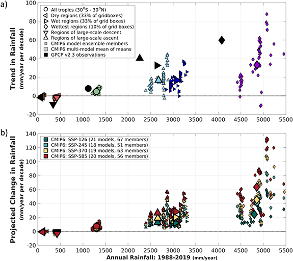
Figure 1. Observed trends (a) and projected changes (b) in the total annual rainfall (mm/year) over several tropical regions, plotted against the reference period (1988–2019) rainfall. The upper panel (a) shows the 32 yr (1988–2019) trend in the monthly anomalies of rainfall averaged over different regions (depicted by various shapes) in GPCP observations (black) and CMIP6 models (green—all tropics, brown—dry regions, red—descending regions, light blue—ascending regions, blue—wet regions, and purple—wettest regions), using joint Historical (1988–2014) and SSP-245 (2015–2019) simulations (18 models, 51 members). The lower panel (b) shows the projected changes in future (2068–2099) rainfall compared to the reference period for four sets of CMIP6 simulations (SSP-126, SSP-245, SSP-370 and SSP-585; different colours) over the same regions (shapes) as depicted in (a). The dry (lowest tercile), wet (highest tercile), and wettest (highest decile) regions are defined by the rank of monthly total rainfall across all tropical (30 °S–30 °N) gridboxes and averaged; regions of large-scale descent and ascent are defined by the corresponding gridboxes with positive and negative monthly mean vertical pressure velocity at 500 hPa, respectively. The ERA5 reanalysis is used to determine the descending and ascending regions for the observations.
Download figure:
Standard image High-resolution imageIn addition to these precipitation-ranked categories, two additional regions are defined based on a simple measure of the corresponding large-scale vertical motion of the gridboxes, the vertical pressure velocity at 500hPa (ω500). For the reanalysis products (ERA5, MERRA-2 and JRA-55) and CMIP6 models, ω500 is bilinearly regridded from the monthly field (from the same dataset); for the observational data (GPCP/CMAP), ω500 are taken from ERA5. Gridboxes with ω500 < 0 are classified as regions of large-scale ascent, while gridboxes with ω500 > 0 are classified as regions of large-scale descent. Finally, the monthly precipitation associated with each region's group of gridboxes is averaged (with area-weighting) to form the time series of average monthly precipitation over each of the regions.
Figure 1(a) summarises the observed (GPCP) and simulated (CMIP6) changes in precipitation during the reference period (1988–2019) for the different tropical regions. Monthly anomalies are computed (by subtracting the monthly means across the 32 years) in order to remove the seasonal cycle, and then linear trends through the 384 monthly anomalies are calculated, with the resulting values plotted as change in rainfall in mm yr−1 per decade. The change in precipitation is displayed against the mean value of rainfall over the same time period (1988–2019), thus the abscissa spans climatologically drier (lower values) to wetter (higher values) regions. The GPCP observations show that climatologically wet regions have been getting wetter over this time period, with annual rainfall increasing ∼34 mm per decade (upper tercile) and ∼60 mm per decade (upper decile); dry-region annual rainfall is seen to be decreasing at ∼2 mm per decade. The CMIP6 suite of historical model simulations exhibit a similar wetting of wet regions and drying of dry regions over this period, albeit at a decreased rate (in the multi-model mean of means). The vast majority of ensemble members simulate increasing rainfall over the wet (and wettest) regions and decreasing rainfall over dry regions, indicating the robustness of an increasing wet-dry contrast in models, which is shown to be in agreement with observations. Figure 1 also indicates that the climatological mean precipitation in wet regions and dry regions is similar to that of large-scale ascent and descent respectively (Emori and Brown 2005, Allan and Soden 2007). Comparable trends are also found, with regions of large-scale ascent wettening and regions of descent drying in both observations and models, consistent with the theoretical paradigm of rainfall to increase in convergence zones and to decrease in subsidence regions in a warming world (Held and Soden 2006, Chou et al 2009, Seager et al 2010).
The analysis of CMIP6 projections (figure 1(b)) simulating the various future scenarios (SSPs) throughout the 21st century, indicates a continuing enhancement of rainfall in wet tropical regions, and a reduction over dry regions; 32 years of rainfall in the latter part of the simulation (2068–2099) is compared with the reference period. Every model ensemble member in the CMIP6 archive that is examined here (see supplementary table 1) shows increasing rainfall in the wet and wettest regions, with larger increases (in general) seen in simulations with higher emission scenarios. The increase in the wettest 10% of gridboxes (per decade) is substantially larger (in both observed trends and climate model projections) than the increase in the broader wet regions.
Tendencies in precipitation in wet and dry regions in GPCP are broadly supported by those in other datasets, despite differences in absolute values and some outliers. The time series of observed annual precipitation (1988–2019) over various tropical regions is summarised in supplementary figure 2, showing the two observational datasets and three reanalysis products. Whilst there is broad qualitative agreement between the various datasets over the different tropical regions, a detailed intercomparison is beyond the scope of the current study. Our analysis therefore focuses hereafter on GPCP precipitation.
The choice of the upper tercile for classifying the wet regions is supported by an analysis of the same CMIP6 simulations across all gridbox rank percentiles (figure 2). Here the annual changes in rainfall are displayed in units of percent change (compared to the reference period) per decade. Decreases over the drier gridboxes are comparable (in %) to the increases over wetter gridboxes. While there are some differences between the individual ensemble members (shown by the thin lines), the multi-model mean (of means) differences (thick lines) between the future and reference periods indicates decreases in rainfall across the lower 60%–70% of gridboxes, and increases across the upper 30%–40%. We henceforth concentrate our analysis on precipitation percentiles split into upper and lower terciles, and analyse the rainfall changes in them separately. However, results are relatively insensitive to defining wet and dry regions using alternative definitions found in the literature (see discussion in Section 4).

Figure 2. Simulated changes in future (2068–2099) rainfall compared to the reference period (1988–2019) from four sets of CMIP6 simulations (SSP-126, SSP-245, SSP-370 and SSP-585). The tropical gridboxes (30 °S–30 °N, n = 3456) are ranked in ascending order of total monthly rainfall (for each month separately), and then averaged to compute the mean rainfall at each rank (for every model ensemble member). Thick lines show the difference (% change in rainfall per decade) in the multi-model mean of model ensemble means; thin lines show the individual ensemble members. The CMIP6 models included are listed in supplementary table 1.
Download figure:
Standard image High-resolution imageThe resulting time series of annual precipitation in wet and dry regions (monthly values smoothed by a 12 month running mean) shows that in model simulations, the rainfall in the wet regions increases from the 1960 s to the end of the 21st century (figures 3(a) and (b)). Although results for individual simulations are noisy, a clear increasing trend is visible and by the middle of the century the annual value of wet-region rainfall in nearly all model simulations is greater than in the reference period (1988–2019). Precipitation in the driest third decreases in the simulations, although the decrease is relatively smaller (than the increase in the wet regions) and by mid-century many annual values still exceed the average rainfall over the reference period. The observed data lie largely but not entirely within the model range, and also show trends of increasing rainfall in wet regions and decreasing rainfall in dry regions (consistent with figure 1).
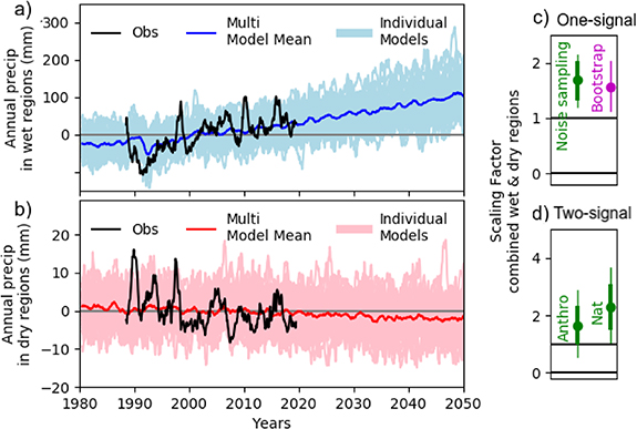
Figure 3. Wet (a) and dry (b) region tropical mean (30 °S–30 °N) annual precipitation anomalies with respect to 1988–2019 (mm) for observations (GPCP—in black) and CMIP6 model simulations (single simulations light blue/pink with multi-model mean in dark blue/red). The model simulations follow the SSP245 scenario from 2015–2100. Wet- and dry-region annual values are calculated as the running mean over 12 months. Scaling factors (right) indicate the magnitude of the multi-model mean fingerprint in observations and are calculated for the combination of the wet- and dry-region mean. Results in (c) are for a one-signal analysis regressing the all-forced simulations onto the observations, using two different analysis methods. 58 model simulations are used in (c) and 51 in (a) and (b) (See table S1 for details). Results in (d) are for a two-signal regression (with 28 simulations used for each signal) and attribute observed changes into anthropogenic and natural contributions, using just the noise sampling analysis method.
Download figure:
Standard image High-resolution image4. Detection and attribution of observed precipitation change
Having shown that the wet regions are getting wetter and dry regions drier it is important to determine whether the observed change is significantly different from changes associated with climate variability and attribute its causes. To do this a detection and attribution analysis was carried out using the multi-model mean fingerprint of precipitation change.
The fingerprint vector was composed of the time-series of wet- and dry-region rainfall over the satellite period, from both climate models (multi-model mean) and observations (as shown in figures 3(a) and (b)). To account for the relative difference in magnitude of the change in the wet and dry regions, both the observations and the model simulations (including the control samples) are standardised by dividing the precipitation in the wet regions by the mean standard deviation (of the wet regions) from all control simulations; similarly the dry regions by the mean standard deviation of the dry regions. This is to avoid the larger magnitude of rainfall in wet regions dominating the analysis. In order to detect the model simulated change in observations, the multi-model running annual mean precipitation from the wet regions joined with the running annual mean precipitation from the dry regions (both for the period 1988–2019) is regressed onto the observations using a total least squares regression (Allen and Stott 2003). Under the assumption of linear additivity of the forcings (which may be affected by responses to atmospheric chemistry, particularly ozone (Marvel et al 2015), however here it is assumed changes are largely unaffected by this in the tropics), the true observed climate response  can be expressed as a sum of the models' responses to individual forcings
  , scaled by respective scaling factors (
 ) (equation (1)). The method accounts for noise due to internal variability in the observations,
  , and in the model response,
  (accounting for the finite ensemble size of the multi-model mean).
As the fingerprint already extracts a robust signal, no optimization has been conducted (see discussion in Polson et al 2013b). A confidence interval for scaling factors describes the range of magnitudes of the model expected signal that is consistent with observations. A model simulated response is considered to be detected if the confidence interval is significantly greater than 0 and is found to be consistent with the observed change if the interval contains 1, since this would indicate that it does not need to be scaled up or down to match the observations. The confidence interval is calculated using two different techniques:
The first method follows Polson and Hegerl (2017) (hereafter noise sampling, following the notation in Delsole et al 2019) and calculates the confidence interval by adding randomly selected samples of pre-industrial control simulations onto the noise-reduced fingerprints of the observations and the model. Each time a scaling factor,  , is recalculated, and a 5%–95% interval is then estimated from the distribution of values. To account for a potential underestimate of variability in model control simulations (see Zhang et al 2007) the confidence intervals are also re-calculated using control samples with doubled variance (as in Polson et al 2013b, Polson and Hegerl 2017). Noise sampling has been critiqued as it may underestimate small, noisy, signals (Delsole et al 2019), although aggregation of results into wet and dry regions should avoid low signal-to-noise ratios. However, in order to address the potential underestimate of uncertainty, a bootstrap method has also been employed. Following Delsole et al (2019), the regression analysis is repeated using arrays formed from the joint time series of wet and dry regions, in the same way as before, but using unsmoothed monthly-values. The confidence interval is calculated by randomly sampling, with replacement, pairs of monthly values from the arrays of observations and model fingerprints to form new arrays the same length as the originals. A new scaling factor is then calculated by regressing the resampled model onto the resampled observations. This process is repeated 10 000 times and a 5%–95% confidence interval is estimated from the distribution.
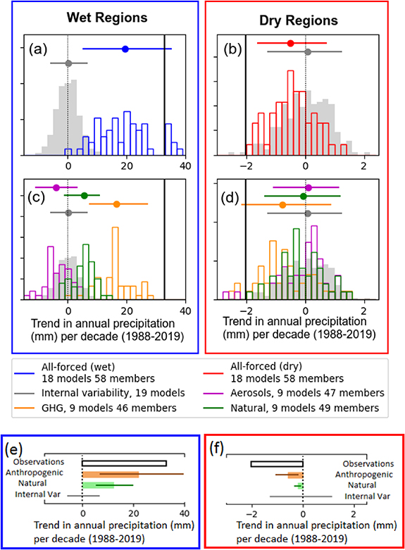
Results show that the historical forced signal is detectable and highly significant irrespective of the method by which uncertainty is estimated, and whether doubling the climate model noise variance (figure 3(c)). The best estimate signal magnitude is between 1 and 2, indicating that to match the satellite data, the multi-model mean simulated precipitation signal needs to be inflated—significantly so in all estimates, consistent with previous studies using CMIP3 and CMIP5 models (Min et al 2011, Polson et al 2013b, Polson and Hegerl 2017). This is supported by figure 4(a) which shows that the observed trends are outside what could be expected from internal variability alone (as sampled by piControl model simulations), in both wet and dry regions and are at the extreme edges of the range in historically forced simulations (see also figure 1(a)). This suggests that the observed change is also larger than individual model simulations.
Figure 4. Normalised histograms of precipitation trends in wet (panels a and c) and dry (panels b and d) regions (mm per decade) over the period 1988–2019. Black vertical line shows the observed trend in GPCP. Histograms show trends in model simulations, with the corresponding horizontal line the 5%–95% range, and the circle the median value. In all panels grey indicates trends in control simulations. The top panels show results for models with all forcings, and the middle panels show results for models with single forcings. Panels e and f show the attributed trends due to only anthropogenic forcings and only natural forcings calculated using the scaling factors from the 2-signal detection and attribution analysis in figure 3(d) to scale the multi-model-mean trends. Wide bars indicate the best estimate and the narrower lines their 5%–95% uncertainty range.
Download figure:
Standard image High-resolution image
Results of our detection and attribution study are broadly consistent when including the data from 1980, although the signal amplitude is even larger early on (supplementary figure 5). Our results are also similar if the analysis is conducted on annual mean values calculated from seasonal means (instead of monthly) as in previous studies (Min et al 2011, Polson et al 2013b, Polson and Hegerl 2017) (supplementary figure 3).
In order to evaluate whether climate model internal variability is consistent with the observed changes, an estimate of the internal variability, ν, in the observations (the residual variability) is calculated by subtracting the scaled model mean results, accounting for the internal variability in the model simulations using equation (2) (following Schurer et al 2015).
where  is the number of model simulations used to calculate the multi-model mean. Supplementary figure 6 shows that the regression residual (equation (1); purple in figure) is within the range of some climate model control simulation trends, although for wet regions, the residual is greater than the mean model variability and is larger than the variability in many of the models. This potential underestimate of the variability in model simulations could result in overly narrow confidence intervals in the noise sampling analysis, and provides justification for our choice to repeat the analysis with control simulations with doubled variance.
Motivated by the expected fingerprint of change in model simulations (figure 2) and following previous work by Polson et al (2013b) and Polson and Hegerl (2017), the wet regions were defined as the wettest third and the dry regions the driest third (see section 3). Other studies have used slightly different definitions, for example Liu and Allen (2013) defined the wet regions as the wettest 30% and the driest regions as the driest 70%, while Gu and Adler (2018) also defined the wet regions as the wettest 30% and dry as the region between 5% and 30%. The detection and attribution analysis has been repeated with these choices as well as several alternatives; the results are found to be insensitive to the precise definition of 'wet' and 'dry' (supplementary figure 8).
We have now determined that there is a significant effect of external forcing on GPCP precipitation. To address the causes of this observed change over the most recent 32 year period requires the analysis of individually forced climate model simulations. Supplementary figure 4 shows that greenhouse gases are expected to have caused a clear wettening trend in wet regions and drying trend in dry regions, both over the historical period (figures 4c and d) and continuing into the future. Anthropogenic aerosol responses show relatively little precipitation change in dry regions, although they show a reduction in wet regions particularly prior to 1980, and a recovery in the second half of the 21st century. However, during the period 1988–2019, the tropics-wide trend due to anthropogenic aerosols is relatively flat (figures 4c and d), suggesting that the response to anthropogenic factors will be dominated by greenhouse gases emissions during this time. The response to natural forcing (which includes changes in solar variability and volcanic eruptions) is also flat apart from a sharp reduction and subsequent recovery in wet regions following historical volcanic eruptions (Agung in March 1963, El Chichon in April 1982 and Pinatubo in June 1991). This is consistent with analysis of volcanic model simulations and detectable decrease in flow in rivers in wet regions (Iles and Hegerl 2015). Note that the timeseries of rainfall in wet regions in GPCP shows a noisy dip around 1991 (figure 3) consistent with historically forced climate simulations. Because Mount Pinatubo erupted early on in our analysis period, recovery from it causes a wettening trend in wet regions (figure 4(c)) which combined with the anthropogenic trend over this period explains the modelled all-forced wettening trend seen in figure 4(a).
In order to determine whether the effect of anthropogenic forcing is detectable or whether the response to natural forcings alone is sufficient to explain the observations, a two-signal multi-linear regression is carried out using multi-model mean fingerprints from model simulations with all forcings and with just natural forcings. Only models which have contributed to both model experiments are used in the analysis which resulted in only 28 simulations for each experiment. From these, scaling factors with confidence intervals are calculated for anthropogenic forcings and natural forcings separately (following Tett et al 2002), and both are found to be detectable (figure 3(d)), confirming a role for both anthropogenic forcings and natural forcings (which will be dominated by the response to the Pinatubo eruption) during this period. Due to the short-term nature of the volcanic forcing, the signal-to-noise ratio is only strong for a small portion of the record; hence, the bootstrap method cannot be used in this analysis. Multiplying the model-mean trend by the calculated scaling factors allows for an estimate of the attributable contribution to the observed trend. Figures 4(e) and (f) shows that wet trends are largely caused by anthropogenic factors with a smaller contribution from natural forcings. The forced contribution to the trend in dry regions is found to be smaller but is still dominated by anthropogenic forcings.
There is some evidence that the response to both forcings is significantly larger in observations than expected from the multi-model mean fingerprint, however due to the large uncertainty in this analysis this conclusion is not significant for the response to anthropogenic forcings in the doubled variance case. Supplementary figure 7 shows that in the regression analysis the scaling factors for the two signals (anthropogenic forcing and natural forcings) have a slight inverse relationship, that is a larger response to natural forcings is consistent with a lesser response to anthropogenic forcing and vice versa, although the response to anthropogenic forcing remains clearly detectible. Thus an anthropogenic scaling factor less than or equal to '1', (indicating that the response to anthropogenic forcings is consistent or smaller than the observed magnitude) is very unlikely and would require that the response to natural forcings is several times larger than the current modelled response. The attribution to anthropogenic forcings is further strengthened by supplementary figure 5, which shows that even if the analysis period commenced later, after the effect of the 1991 Pinatubo volcanic eruption had dissipated (e.g. after 1994), the historical change would still be detectable in observations.
5. Conclusions
In summary, there is a clear and detectable sharpening of the contrast between wet and dry regions in blended satellite/in situ precipitation records, which follows expectations from climate model simulations and is supported by process understanding of increased rainfall over ascending regions. The effects of natural and anthropogenic forcings are both detectable with the largest contribution likely due to greenhouse gas increases, with a smaller and shorter-lived increase due to the recovery from the Pinatubo eruption of 1991. However, detection and attribution results show a larger response to these external forcings in observations than expected from the multi-model mean simulations. The observed drying trend in dry regions is also larger than in all individual historically-forced simulations, whereas the observed increasing trend in wet regions is stronger than in all but 8 out of 58 model simulations (all from only two out of 18 models). This might be partly related to a stronger rainfall response to volcanism (see also Iles and Hegerl 2015) but our results also support a stronger than modelled response to anthropogenic forcings. This could potentially indicate an underestimate of rainfall change in many climate models, but there might also be a role of observational uncertainty. Our results provide powerful evidence that the expected signal of an intensification of the low-latitude water cycle is already underway, and may be larger than expected. In order to make this result regionally relevant, changes in circulation and effects of regional influences over land need to be better understood.
Acknowledgments
Early work on this was supported by the ERC funded project TITAN (EC-320691), and AS and GH under the UK NERC under the Belmont forum, Grant PacMedy (NE/P006752/1). GH and AB were supported by the H2020 project EUCP (776613). GH and AF were supported by the Hans Sigrist foundation through the Sigrist Prize 2015.
We thank D Polson for code and R Allan and P Stott for discussion. The authors acknowledge the World Climate Research Programme's Working Group on Coupled Modelling, which is responsible for CMIP, and thank the climate modelling groups for producing and making available their model output. For CMIP the US Department of Energy's Program for Climate Model Diagnosis and Intercomparison provides coordinating support and led development of software infrastructure in partnership with the Global Organization for Earth System Science Portals. This work used JASMIN, the UK collaborative data analysis facility
GPCP was produced as part of the Global Energy and Water Cycle Exchanges (GEWEX) effort under the World Climate Research Program (WCRP). MERRA-2 is an official product of the Global Modeling and Assimilation Office at NASA GSFC, supported by NASA's Modeling, Analysis, and Prediction (MAP) program. ERA5 and ERA-Interim were produced by ECMWF. Copernicus Climate Change Service (C3S) is implemented by ECMWF on behalf of the European Commission. JRA-55 was produced by JMA.
Data statement
Data used in this study is publicly available from the following sources:
CMIP model output is available at: http://pcmdi9.llnl.gov/.
The GPCP and CMAP data were provided by the NOAA Office of Oceanic and Atmospheric Research (OAR) Earth System Research Laboratory (ESRL) Physical Sciences Division (PSD). The ERA5 output (downloaded at 0.25°× 0.25° resolution for precipitation and 2.5° × 2.5° for other variables) is available from the Copernicus Climate Change Service (C3S) Climate Data Store. The MERRA-2 output (downloaded at 2.5°× 2.5° resolution) is available from the Goddard Earth Sciences Data and Information Services Center. The JRA-55 output (downloaded at 1.25°× 1.25° resolution) was provided via the JMA Data Dissemination System (JDDS).
All analysis code will be made available on request.