

Abstract
Studies on the impact of climate change in lakes have mainly focused on the average response of lake surface temperature during three summer months (July, August, September, usually termed JAS). Focusing on the Laurentian Great Lakes, we challenge this common assumption by showing that the thermal behaviour is diversified in time both among different lakes and within a single one. Deep regions experience a stronger warming concentrated in early summer, mainly due to anticipated stratification, while shallow parts respond more uniformly throughout the year. To perform such analysis, we use the difference between the five warmest and coldest years in a series of 20 years as a proxy of possible effects of climate alterations, and compare the warming of lake surface temperature with that of air temperature. In this way, based on past observations obtained from satellite images, we show how the warming is heterogeneously distributed in time and in space, and that the quantification of lakes' thermal response to climate change is chiefly influenced by the time window used in the analysis. Should we be more careful when considering averaged indicators of lake thermal response to climate change?
Export citation and abstract BibTeX RIS

Original content from this work may be used under the terms of the Creative Commons Attribution 3.0 licence. Any further distribution of this work must maintain attribution to the author(s) and the title of the work, journal citation and DOI.
1. Introduction
Lakes are considered as 'sentinels of climate change' [1, 2], thus making the study of their thermal trends particularly informative to gather insights on how inland water resources respond to evolving climate conditions [3–6]. A number of studies compared the rates of increase in lake surface water temperature (LSWT) with those in air temperature (AT), often finding the surprising result that water is warming faster than air in summer months [7–9]. A particularly rapid LSWT warming has been found for deep and cold lakes [10, 11], where an earlier onset of stratification due to rising AT is expected to produce an amplified LSWT warming in summer, through reducing the long adaptation timescale between LSWT and AT anomalies (i.e. thermal inertia) of these lakes [12, 13]. Other explanations have been proposed for this amplified response, including variations to the large-scale climatic forcing, solar radiation [14], lake water clarity [15], and timing and duration of ice cover [7, 10]. However, one may wonder to what degree the quantification of this observed amplified trend is influenced by the methodological approach used in the data analysis.
To date, most studies on lake temperature assumed AT as a simple proxy of climate change and introduced synthetic indicators to quantify LSWT response to changes in climate [16]. Several significant works on this subject focused on the response of LSWT to AT during three summer months: July, August and September (JAS). The use of these three months (instead of other combinations or single representative months) to describe the summer period was originally proposed by Austin and Colman [7], and later presented with the acronym JAS by Schneider et al [8]. Since then, as a technological lock-in, this period (and the corresponding January, February and March JFM period for lakes in the southern hemisphere) has become the standard for most of the following analyses, including recent comparisons on a global scale [10, 11, 17].
Furthermore, most of the research on lake warming was based on correlation analyses between concurrent variations of AT and LSWT [18], without explicitly considering that LSWT at a given time is inherently influenced by the development of lake thermal stratification [13, 19]. In turn, stratification is the result of the previous history of the system, and can differ among lakes as it is chiefly controlled by thermal inertia, external forcing, and morphometric characteristics [5, 12]. Hence, regressions between concurrent AT and LSWT may be not physically significant, or at least not exhaustive, especially in those lakes that are characterised by large depths, hence large thermal inertia. Rather, the antecedent variation of AT is a leading factor controlling LSWT dynamics and should be considered extending back early before the period when LSWT is examined [7, 13, 20, 21]. How to properly define the extension of the significant AT time window depends on the evolution of stratification and the thermal regime of the lake at hand. The interaction among physical mechanisms controlling lake thermal dynamics is still object of investigation [11, 22–25], thus an operational definition of such time window is not clear-cut.
Recent contributions have started to highlight the limitations of using seasonal metrics of LSWT, such as the JAS average, to characterise the response of lakes to climate change. For instance, by analysing six shallow and small lakes in Wisconsin, the existence of substantial differences in monthly LSWT warming rates was shown [16], demonstrating that JAS or annually averaged trends do not fully represent the effects of climate change on lake temperatures. Similarly, large intra-annual variability in warming rates emerged from the analysis of Central European lakes of variable size and located in different climate regions [26–28], and also from the analysis of historical and projected LSWT in the deep Lake Tahoe (USA) [29].
In addition to considering time-averaged metrics, it is also common practice to analyse lake-averaged values or single-point measurements of LSWT. However, LSWT dynamics are significantly affected by the local depth, which in natural lakes is also a proxy for the distance from the shores. This is particularly evident in large deep lakes, where spatial patterns due to differential warming may occur [21, 30–32].
Therefore, some questions arise and need to be addressed: Are JAS-based indicators the best choice to detect the effects of climate change on LSWT? Are other options more suitable to highlight specific dynamics depending on the type of lake and on the climate region? Is it always reasonable to analyse concurrent AT and LSWT dynamics, or may it mystify the correct interpretation of the investigated phenomena? In general, should we be more careful when considering temporally and spatially averaged indicators of lake thermal response to climate change?
In order to answer these questions, we focus on the Laurentian Great Lakes (Superior, Michigan, Huron, Ontario, Erie, located between USA and Canada). They have been the subject of several studies about the thermal and hydrological response to changing climatic conditions [13, 20, 21, 33–36] because of their scientific, ecological and economical relevance. Considering also the large amount of available data, their markedly different bathymetries, and the fact that they span almost 6° of latitude, they represent an ideal case study to understand the spatial and temporal response to the current warming trends [37–39]. Referring to daily LSWT maps retrieved from satellite imagery [40] and to large-scale AT dynamics obtained by re-analysis, we performed a 'natural experiment' [41] looking at the historical dataset and separating warm and cold years. We interpreted the difference as a possible description of the effects of the future warming and analysed them to characterise the thermal behaviour of the different lakes and their LSWT spatial gradients, an original approach with respect to most studies that focused on (linear, in most cases) trends.
2. Methods
2.1. Study site and datasets
The Laurentian Great Lakes cover an area of 244.106 km2, with a North–South extension of more than 800 km (detailed features reported in the supporting information is available at stacks.iop.org/ERL/15/034060/mmedia). Lake Superior is the deepest, largest, and most northern lake with a stratified period that normally begins in June and a maximum water temperature that normally does not exceed 17 °C. At the other extreme, Lake Erie is the shallowest, smallest (in terms of volume), and most southern lake, with stratification beginning already in April and maximum water temperatures of almost 25 °C.
The analysis of AT and LSWT was based on two records that simultaneously cover the period 1995–2014 (20 years). The spatial description of daily values of LSWT was obtained from GLSEA maps (provided by National Oceanic and Atmospheric Administration, NOAA, Great Lakes Environmental Research Laboratory, GLERL—see the section 'Data availability' at the end of the article), retrieved from satellite images. At the same time scale, AT was derived from re-analysis ERA-Interim data (provided by the European Centre for Medium-Range Weather Forecasts, ECMWF—see 'Data availability'), computed 2 m above the ground. The bathymetric data of the five lakes (figure 1) were retrieved from the shape file available in NOAA website and then interpolated on a regular grid.
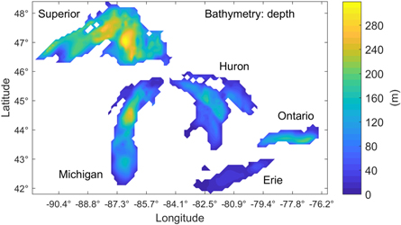
Figure 1. Bathymetry of the Laurentian Great Lakes.
Download figure:
Standard image High-resolution imageLSWT data were aggregated on a regular 12.5 × 12.5 km grid, while AT values were lake-averaged. Details on the procedure are provided in the Supporting Information. In the present analysis, we rely on the official validation of the remotely sensed measurements against actual values of LSWT as provided by NOAA, hence here we do not discuss (nor question) how technical issues such as, e.g. the atmospheric correction on the remotely sensed data, or the conversion of skin temperatures to 'bulk' near-surface temperatures have been tackled. Similarly, we rely on the accuracy of AT estimates by ECMWF re-analysis, whose performance has been well documented in previous dedicated studies [42, 43]. In this respect, since our analysis is comparative, being essentially based on the use of temperature anomalies, possible systematic biases in AT or LSWT estimates are not expected to affect the results significantly. Indeed, even though the reconstructed data may not exactly correspond to the actual LSWT or AT values, the two datasets are internally coherent. Possible time-varying or temperature-dependent errors may also exist, which however are difficult to assess and correct. Nevertheless, these datasets have been widely used in several limnological applications, both for NOAA's LSWT [20, 21, 23, 31] and ECMWF's AT [6, 28, 44, 45], which confirm their validity and reliability.
2.2. Definition of averaged indicators
In order to characterise the typical annual thermal dynamics of a lake, we use the term 'climatological year' to refer to the 365 d cycle of LSWT and AT obtained by averaging the temperature for each day of the year (DOY). Hence, for a series of Ny years, the annual cycle of temperature  is defined as:
The 29 February of leap years was not considered in this computation. Since we focus on the lake response to large-scale climatic variations, and not to local atmospheric conditions, for AT we considered lake-averaged values of  .
.
In addition to the average climatological year, we computed also the 'cold' and 'warm' reference years for each lake, respectively by considering only the five coldest and warmest years in the whole series. The selection of these years was based on the annual means (1 January–31 December) of lake-averaged LSWT (figure 2(a)). Averaging among the five lakes provided the cold years (1996, 1997, 2003, 2009, 2014) and the warm years (1998, 2005, 2006, 2010, 2012) used in the following analysis. This allowed us to investigate the spatial distribution of the LSWT differences between the warm and cold years, as a proxy of the effect of a change in climatic conditions.

Figure 2. Time series of annual averaged temperatures ((a): LSWT, (b): AT) with the indication of the five coldest and warmest years. The black thick line shows the mean among the five lakes. Numbers represent the last two digits of the year. All temperature values are lake-averaged.
Download figure:
Standard image High-resolution imageAn equivalent selection based on annual means of AT would have provided a consistent identification of cold and warm years (figure 2(b)), with the only difference of the inclusion of 1999 instead of 2005 within the warm years (LSWT differing less than 0.4 °C on average). More details on the selection procedure and on the possible influence of alternative criteria are discussed in the Supporting Information.
The temperature (either LSWT or AT) difference was used to characterise the thermal behaviour of the different lakes, and to gain some indirect insights of how the systems could respond to a warming climate in the future. Hence, we defined

where T stands for either LSWT (in each cell) or AT (lake-averaged), and  and
and  indicate the reference years defined considering the five warmest and coldest years, respectively (i.e. Ny = 5 in equation (1)). The underlying assumption of using
  and
and  is that the thermal memory of the lake system is short enough that each year can be considered as independent. This was demonstrated to be valid for Lake Superior by showing that the effect of varying AT conditions in January on subsequent LSWT dynamics vanishes after August [13]. If this has been observed for Lake Superior, which is the deepest lake (hence the one with the largest thermal inertia), it is verified for all the five Great Lakes. Additionally, this was further corroborated by Zhong et al [20], who showed the minor role of declining ice cover (a proxy of winter conditions) in the rapid warming of the Great Lakes.
In order to quantify LSWT response of a lake to changes in AT (here assumed as a general proxy of climatic conditions), we defined a suite of indicators, which are described in the following paragraphs.
First, we considered a general time-averaged ΔT(period) obtained by averaging the temperature difference ΔT in equation (2) over different periods of the year, the general definition being:

where D1 and D2 are the first and last DOY considered in the averaging period and Nd = D2 − D1 + 1 is the corresponding length expressed in number of days. As an example, the period JAS is characterised by D1 = 182, D2 = 273, and Nd = 92. Equation (3) is used to temporally average both local and lake-averaged temperatures.
Second, we introduced a simple lake-averaged indicator, hereafter defined as 'warming efficiency':

where  is the lake-averaged LSWT increase between the warm and cold reference years for a given period2 (time averaging window, e.g. JAS) produced by the change of ΔAT in period1. Note that the two averaging periods can coincide or, more generally, can be different. It follows that LSWT warms as much as AT when η = 1, LSWT response is damped when η < 1, whereas when η > 1 the warming of LSWT is amplified with respect to that of AT.
Third, we used two different definitions of the maximum LSWT differences (see the conceptual sketch in the supporting information). As a first indicator, we defined the maximum value of the LSWT difference (i.e. the maximum difference of temperature considering the same DOY in the warm and cold years):

where we recall that LSWT is defined in each cell k. Connected to this, for each cell k we also computed the DOY in which the largest change of LSWT occurs,  . As a second indicator, we defined the difference between the maximum values of LSWT in the warm year and in the cold year:
For each cell k, we also defined the indicator ΔDOY(LSWTmax) indicating the time lag between the occurrence of LSWTmax in the warm relative to the cold reference year.
Finally, the strength of thermal stratification was estimated by means of the dimensionless parameter δ, defined by Piccolroaz et al [46] as the ratio between the volume of the lake surface layer participating to the heat exchanges with the atmosphere (i.e. approximately the epilimnion) and the entire volume when the lake is completely mixed (see also the supporting information). The surface layer depth (SLD) was estimated by multiplying the variable δ by the average depth of the lake [12]. Low values of δ indicate a strong thermal stratification, typical of the summer period, when the response of LSWT is accelerated by the lower water volume reacting to changes in AT. Conversely, the thermal inertia is maximum for δ = 1 when almost the whole water column is affected by the heat exchange at the lake surface.
3. Results
3.1. Thermal characterisation of the Great Lakes
The morphology of the Great Lakes and the climatic variability that they experience across different latitudes influence LSWT dynamics. On the one hand, the five lakes are characterised by different depths. The lake s volume determines its heat capacity, while the most important heat fluxes scale with the lake s surface area. Hence, the thermal inertia, the 'memory' of the system, is controlled by the averaged depth: the larger the depth, the slower the adaptation to external forcing. On the other hand, the large geographic extent of the Great Lakes region encompasses a variety of local climate conditions, primarily depending on latitude [47]. As a first approximation, these conditions can be associated with AT (figure 3(a)) because air warms as a result of the combination of all climatic factors (e.g. solar radiation depending on latitude). The combination of these two effects produces different LSWT cycles (figure 3(b)) and stratification dynamics (figure 3(c)) in the five lakes.
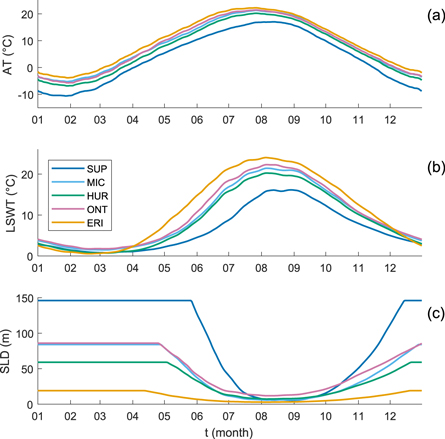
Figure 3. Climatological years for AT (a) and LSWT (b) computed with the whole records of data (1995–2014), and temporal evolution of the surface layer depth (c), which is dependent on the thermal inertia of the lake in stratified conditions. All temperature values are lake-averaged.
Download figure:
Standard image High-resolution imageThe onset of stratification is particularly important for summer temperatures in deep lakes because it reduces the volume of water affected by the surface heat fluxes, thus causing a faster increase of LSWT [13]. For instance, the rate of LSWT change in Lake Superior experiences an acceleration as soon as the SLD decreases in late spring (around the end of June, figure 3(c)). Such a behaviour is not so evident in the other, shallower, lakes (especially in Lake Erie) where the intra-annual variability of the SLD is relatively smaller and the transition to stratified conditions is not so sudden (figure 3(c)). The time lag of the onset of stratification with respect to the peak of the warm season is therefore one of the key elements controlling the warming trends resulting from changing climate conditions [11]. Indeed, it chiefly controls speed and rate of response of the lake to varying external conditions.
Besides inter-lake heterogeneity in the thermal response, significant intra-lake spatial patterns of LSWT exist as well [21, 31, 48], primarily affected by the bathymetry, which deepens moving from the coast to the interior (figure 1). However, also the role of latitude can be clearly recognised looking at the local maximum values of LSWT (figure 4(a)) especially in Lake Michigan, which is elongated in the north–south direction. Modulated by seasonal stratification, local depth concurs to determine the SLD and hence the thermal inertia, which in turn controls the LSWT response. This behaviour is visible in the DOY when the maximum temperature occurs (figure 4(b)). Deeper and northern locations show a significant delay (approximately one month) with respect to the early warming of the southern shallower Lake Erie.
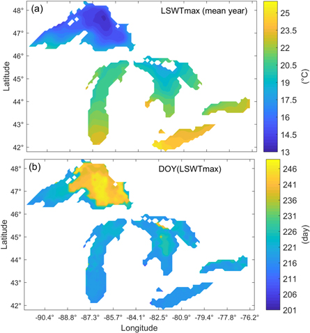
Figure 4. (a) Map of the daily maximum LSWT values (°C), LSWTmax, for the climatological year obtained from the whole record of data. (b) Day of the year (DOY) when it occurs.
Download figure:
Standard image High-resolution image3.2. Spatial distribution of the warming
The maximum LSWT difference,  , reaches values up to 13 °C in the deep regions of Lake Superior (figure 5(a)) and 10 °C in those of Lakes Michigan, Huron and Ontario. Much lower values (less than 6 °C) occur in Lake Erie and in the shallower regions of all lakes. Such a depth- and latitude-dependent spatial distribution can be explained by referring to the change in stratification timing between cold and warm years. In the deep and northern regions, both the onset and the strongest stratification conditions occur earlier, lowering the thermal inertia already at the beginning of the warmest period (for AT), and eventually determining an enhanced LSWT increase. The spatial distribution of the DOY when the
  occurs (figure 5(b)) varies from July, in Lake Superior and in some deep parts of Lakes Michigan and Huron, to May–June in the shallow regions and in Lake Erie.
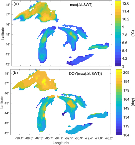
Figure 5. (a) Map of the maximum difference of temperature (°C),  , between the warm and cold climatological years. (b) DOY when the maximum difference occurs.
Download figure:
Standard image High-resolution imageHowever, the  is not necessarily the most meaningful parameters to consider. It is affected by the time shift in lake response and accounts for the period of the year when the largest difference occurs, but the actual maximum LSWT through the year might remain unchanged, or even decrease. In order to complement the analysis, we computed the spatial distribution of the difference in the annual maximum temperature, i.e. ΔLSWTmax (which is lower than
  ). The analysis of the spatial map of ΔLSWTmax (figure 6) confirms the results discussed above. Lake Superior clearly appears as a hotspot in this case, with differences up to 7 °C in the deepest regions (figure 6(a)). The difference in other lakes did not reach 4 °C, with Lake Erie mostly below 2 °C. The change in the DOY of maximum LSWT, ΔDOY(LSWTmax) (figure 6(b)) is negative almost everywhere, denoting an anticipation of LSWTmax, as expected. However, the DOY is not significantly modified in Lake Erie and in the shallow regions of the other lakes, while it is anticipated of more than one month in the deep regions of Lakes Superior and Michigan (and, to a lower extent, of Lake Huron and Ontario).
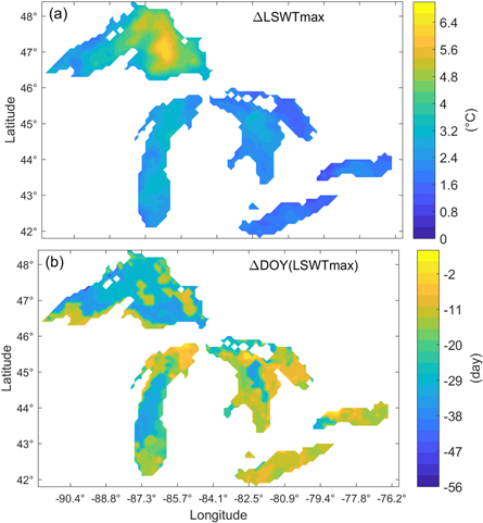
Figure 6. (a) Map of the difference between local maximum LSWT (°C), ΔLSWTmax, obtained for the reference warm and cold year. (b) Variation (in days) of the period when the maximum value occurs.
Download figure:
Standard image High-resolution imageThe spatial variability in the LSWT response is strictly connected to the degree of variability in the lake bathymetry. In other words, the local depth does influence the thermal dynamics significantly: LSWT increases more in deeper regions than along the shores, because in these regions the changes in timing and strength of stratification are larger. This behaviour is summarised in figure 7, where the local LSWT differences (both  and ΔLSWTmax) are correlated with the corresponding local depth. The maximum LSWT difference,
  , shows a clear dependence on depth (figure 7(a)), with a constant growth from 3 °C to 13 °C from shallow to deep regions, irrespective of the lake considered. A similar dependence is evidenced by the difference in maximum LSWT, ΔLSWTmax , but with a smaller range of variation (figure 7(b)). While the highest warming does not exceed 7 °C, a lower asymptote can be recognised at about 2 °C.

Figure 7. (a) Maximum difference of LSWT,  , and (b) difference in maximum temperature, ΔLSWTmax, between the warm and cold climatological years as a function of the local depth (in logarithmic scale), as obtained from figures 5 and 6, respectively.
Download figure:
Standard image High-resolution imageFinally, in order to follow the temporal dynamics more in detail, we plotted the monthly averaged LSWT difference between the warm and cold reference years in figure 8. It is immediately clear that the southern lakes and the southern shores of Lake Superior warm earlier (May), with maximum values in Lake Michigan, Huron and Ontario in June. After that, the warming decreases almost everywhere except for Lake Superior and the deepest regions of Lakes Michigan and Huron, reaching the maximum difference in July. In the deepest parts of Lake Superior the strong warming lasts until August. The sequence of the spatial distribution of daily LSWT differences between warm and cold years is provided as a video in the Supporting Information.
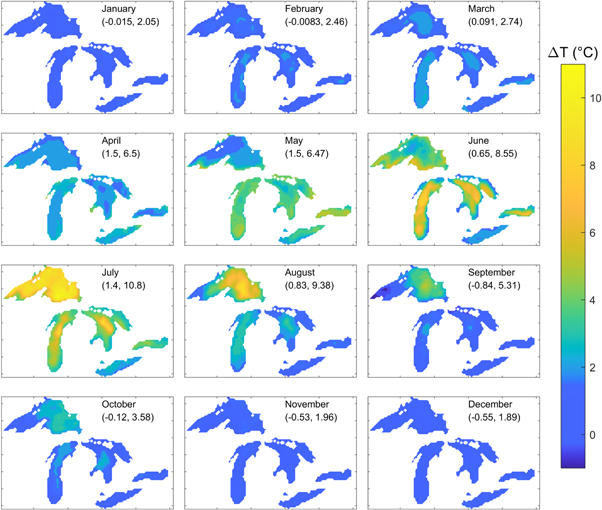
Figure 8. Monthly averaged difference of LSWT between the warm and cold climatological years. Minimum and maximum values (°C) are reported between parentheses in the subplots' titles. A nonlinear colour map is used to enhance the lower range of temperature difference.
Download figure:
Standard image High-resolution image3.3. Lake-averaged response to warming
It is now useful to look at lake-averaged values of AT and LSWT in order to better focus on their temporal variability. The AT in the warm reference year is obviously higher that in the cold one (figure 9(a)). LSWT shows even more evident differences (figure 9(b)), characterised by an amplified warming response in late spring and summer. As already discussed, this is directly related to the timing of the thermal stratification (summarised by the dimensionless parameter δ for a clear comparison among lakes with different depths), which is different for the five lakes and is anticipated in the warm years compared to cold years (figure 9(c)). The difference is particularly visible for Lake Superior, where the stratification starts almost one month in advance and the maximum LSWT increase is greatly amplified.
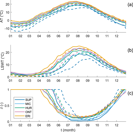
Figure 9. Climatological years for AT (a) and LSWT (b), computed separately considering the five warmest (solid line) and coldest (dashed line) years. (c) Parameter δ representing the strength of stratification (dimensionless depth of the surface layer). All temperature values are lake-averaged.
Download figure:
Standard image High-resolution imageThe explicit differences between the warm and cold reference years are shown in figure 10. The increase of AT experienced by the different lakes is not the same (figure 10(a)), with a stronger warming in Lake Superior and a milder one in Lake Erie. The AT warming is far from being constant throughout the year: looking for simplicity at the average among the five lakes (thick black line), it is possible to observe a larger warming (approximately 4 °C) from late January to mid April, some oscillations in summer, and almost no change in autumn. Interestingly, the mean increase of AT is on the same order as the asymptote detected in figure 7(b).
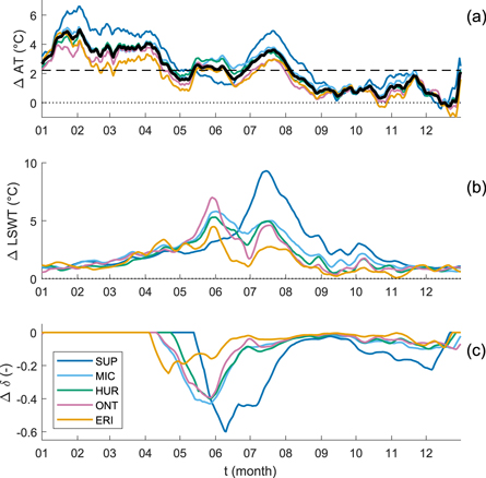
Figure 10. Differences for AT (a), LSWT (b), and δ (c), between the warm and cold climatological years shown in figure 9. The black thick line in panel (a) shows the mean AT among the five lakes; the black dashed line shows the annual mean (ΔAT = 2.22 °C).
Download figure:
Standard image High-resolution imageThe decreasing trend in the AT differences throughout the year produces a complex response of LSWT (figure 10(b)), which is markedly different in the five lakes. The response is stronger and occurs later in Lake Superior (ΔLSWT reached almost 10 °C in July), while Lake Erie shows a smoother and earlier LSWT increase (ΔLSWT of less than 5 °C in late May). The behaviour of the other three lakes is intermediate between those two extreme cases, but in all cases the maximum LSWT difference is always much larger than AT differences.
Lake Superior is the only lake showing a single large peak in ΔLSWT, centred in July, while all the other lakes experience also another distinct warming period at the end of May. This can be partially attributed to the fact that also ΔAT is smaller in May for Lake Superior compared to the other lakes. More important, however, is the different way the five lakes experience the anticipation of the stratification onset in the warm year compared to the cold year, which is shown in figure 10(c) (where, in analogy with equation (2),  ). In contrast to the other lakes and due to the larger thermal inertia, the heat excess stored in Lake Superior during winter and early spring is not sufficient to anticipate the strong thermal stratification in May, when the first AT warming peak occurs. The consequence is the absence of any visible amplified response of LSWT to the peak in ΔAT. Rather, this period coincides with the onset of thermal stratification, one month earlier than in the cold year. The steady warming of the lake that starts in winter continues until mid June, together with a progressive strengthening of the thermal stratification. After mid June, a marked LSWT warming occurs, with a large peak in July. This peak coincides with the period when the maximum stratification is reached (see figure 9(c)) and occurs exactly in correspondence of the second ΔAT peak.
It is significant that, in the other lakes, the largest ΔLSWT does not coincide with the largest warming in AT (July), rather it occurs in the period with the strongest change in thermal stratification (end of May). As we have seen, the amplification of LSWT warming compared to AT is essentially determined by the earlier development of strong stratification [11, 13]. This suggests that it is generally erroneous to describe LSWT dynamics by simply infer a direct influence of AT on LSWT, since thermal stratification does actually play a central role and must be accounted for. It is also erroneous to simply relate LSWT changes to concurrent AT changes, as thermal stratification is chiefly influenced by the conditions experienced by the lake during previous months, especially in deep lakes with large thermal inertia, as already noted by Zhong et al [21]. Building on these considerations, in the next section we challenge the appropriateness of using time-averaged indicators for LSWT and AT to describe lake thermal dynamics.
3.4. Sensitivity to warming described by time-averaged indicators
We have seen that the lake thermal response is characterised by a complex temporal dynamics, so two fundamental questions arise: Can we describe the LSWT warming in a simplified way, for instance by means of time-averaged indicators? Which time window should be used for AT warming to properly quantify and predict its effect on LSWT in a given period? To address these questions, we refer to different time windows: the conventional July–August–September (JAS) period, which is typically considered in analyses of summer warming in lakes [10, 11, 17, 21, 31, 49], the period May–June–July (MJJ), the annual mean, and the single-month averages from April to September. We notice that JAS has the first month coincident with the period of maximum LSWT response in Lake Superior (i.e. July). Consistently, MJJ has been chosen as counterpart as it has the first month coincident with the period of maximum LSWT response for all the other lakes (i.e. May, see figure 10(b)).
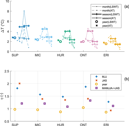
We computed the lake-averaged temperature differences for LSWT and AT (warm-cold years) in the time-averaging windows listed above (figure 11(a)). Annual averages are approximately constant in the five lakes for both LSWT (circles) and AT (crosses). On the contrary, significant variations are shown by monthly (i.e. from April to September) and seasonal (JAS and MJJ) averages. We estimated the corresponding warming efficiency η (equation (4)) for four significant periods: in three cases using concomitant temperature differences (year, MJJ, JAS) and in the last case comparing the LSWT change in JAS with the AT change in a longer period from March to August (figure 11(b)).
Figure 11. (a) Time-averaged temperature differences (LSWT and AT) considering monthly means (from April to September), seasonal means (MJJ and JAS), and annual averages. (b) Warming efficiency, η, considering mean LSWT and AT for different periods (MJJ, JAS, and year for both AT and LSWT; and March to August for AT and JAS for LSWT). Plotted points are shifted to increase readability.
Download figure:
Standard image High-resolution image
What we can learn from the analysis of the warming efficiency is that the five lakes behave similarly for the annual averages (circles in figure 11(b)), with values of η ∼ 1. The weakest response is observed for Lakes Huron and Erie, while the strongest is for Lake Ontario. Interestingly, in this case Lake Superior does not stand out as a hotspot. The peculiar behaviour of Lake Superior emerges when looking at other indicators. In this lake, the values of η evaluated based on JAS (red×) and on MJJ (blue+) are much higher than in the other cases, with values approaching 2. This means that LSWT warms twice AT. This behaviour is particularly visible for η based on JAS, and is due to the large increase in LSWT observed in July, markedly amplified by the strong stratification in that period (see previous section and description of figure 10). In turn, due to the long memory of the system, the earlier development of strong stratification is chiefly determined by previous AT conditions. One may therefore wonder whether concurrent averaging windows for LSWT and AT are appropriate, and consider evaluating η by assuming JAS for LSWT and a longer period as averaging windows for AT. The length of the AT averaging period should be taken according to the lakes' thermal inertia, thus in principle different lengths should be considered for shallow and deep lakes. In the present analysis, for simplicity, we assumed the MAMJJA period from March to August (see purple squares). Looking at this indicator, the story changes dramatically: Lake Superior behaves similarly to the other lakes, and the strongest warming can be attributed to Lake Ontario.
It is also important to note that η evaluated based on JAS (red×) is smaller than the corresponding indicator evaluated based on MJJ (blue+) for all lakes apart from Lake Superior. This is coherent with the analysis of figure 10 presented in the previous section, whereby these lakes experienced the largest LSWT warming in late May and in presence of a smaller ΔAT compared to July. Relevant is the large value of η based on MJJ for Lake Ontario, which approaches 2 as in Lake Superior and thus indicates that also this lake might be classified as a hotspot. However, this distinctive behaviour only emerges looking at MJJ, but does not characterise the JAS period. This clearly suggests that JAS is not necessarily the proper period to detect the strongest warming episodes in lakes that are not as deep as Lake Superior (mean depth 146 m, the 28th deepest in the world). Shallower lakes (as, for instance, the other four Great Lakes, with a mean depth in the range 20–90 m) are the most numerous in the world, so we claim that, in most of the cases, the use of JAS-based indicators can mystify the description of the warming dynamics, being not fully exhaustive and universally representative.
4. Discussion
4.1. Methodological approach
In this study, we implemented an approach that is unusual in limnological studies of lakes' thermal dynamics and response to climate change. We selected warm and cold years from long historical records, computed the reference (climatological) years for the two sets, and evaluated the temperature differences. This approach allowed for retaining both the temporal variability, which is embedded in the time series, and the spatial distribution, which depends on the source of data and is particularly well resolved in remotely sensed data.
We found that the increase of AT between the cold and the warm reference year was 2.2 °C on average (see section 3.3), a value that falls within the range (1 °C–4 °C) of the expected climate warming in the 21st century [50]. As a response to this AT warming, we observed how LSWT changes with non-uniform temporal and spatial patterns. We assume that the same qualitative response will characterise the lake thermal dynamics in the future, and we claim that the results of the present analysis can be interpreted as first-order quantification of how LSWT in the Great Lakes is likely to change in the next years. These results represent a verifiable hypothesis over the next decade.
The proposed approach differs from most of previous analyses, which focused on evaluating long-term rates of AT and LSWT [7, 10], in particular by using linear trends [8, 9, 16]. Two limitations are implicit in the latter approach. First, how meaningful is a linear trend for understanding the physical response of LSWT to climatic warming? This is especially critical when LSWT is characterised by a certain periodicity that is not known a priori and is possibly associated to a time scale longer than the available time series. In this regard, some authors [28, 29] already warned about the use of simple linear trends highlighting several problems. First, because linear trends can mask the occurrence of interannual fluctuations, anomalous interdecadal warming/cooling periods, and regime shifts, and thus affect greatly the interpretations of the underlying mechanisms that are responsible for long-term changes. Second, linear trends are generally evaluated based on time-averaged indicators for LSWT and AT, for example considering the JAS months as an averaging period. However, as Winslow et al [16] advocated and we have thoroughly demonstrated, the choice of JAS is not neutral when the goal is to quantify the critical conditions in the most general case. Climate warming has numerous effects on the thermal structure of the water column, which in turn controls the phenology of ecological processes in lakes [51, 52]. Therefore, we should be careful and look for indicators that better summarise thermal dynamics effects.
4.2. Is JAS the best period to detect climate change effects?
It is evident that the five Great Lakes are expected to react in different ways to climate warming, with large inter- and intra-lake variability, depending on latitude and depth distribution. The analysis of the LSWT differences that occurred between the warm and the cold years showed that LSWT is both temporally and spatially distinct. Warmer years are characterised by an anticipated spring/summer warming in shallower areas and more pronounced LSWT variations in deeper areas, mainly due to changes in the timing of stratification. In fact, in the deep and northern regions, both onset and strongest stratification conditions occurred one month earlier (June instead of July, and July instead of August, respectively, see figure 9).
Our analysis confirms the concern about Lake Superior as a hotspot for LSWT warming [7]: this lake presented the largest warming efficiency η in JAS among the five, and LSWT warmed almost twice as much as AT. In the deep Lake Superior, a significant contribution to JAS-averaged LSWT is due to the AT warming in previous periods (spring, and even winter), and not only to JAS-averaged AT, through a process already highlighted in recent literature [13, 20]. Using the JAS-based indicators, the other lakes did not appear to be significantly affected by climate warming as Lake Superior, showing lower values of η ≃ 1.4 for Michigan, Huron, Ontario, and <1 for Lake Erie (figure 11(b)).
However, additional complexity is introduced when considering, for instance, the MJJ-based indicator. While Lake Superior still presents similar (large) values of η in MJJ, the response is enhanced in other lakes (Ontario, in particular), which show much higher (close to 2) values of η. Considering a longer period (March to August) for AT changes to compute η for LSWT changes in JAS, the picture becomes even more interesting, with Lake Superior behaving similarly to the other lakes, and the effect resulting more pronounced in Lake Ontario.
This is a clear evidence that the period considered for assessing the response to a warming climate is not neutral. Some lakes will have larger reactions in summer, while for others the strongest response will occur in late spring, so the JAS metric might lead to erroneous conclusions. In this respect, previous studies using the JAS metric may not adequately represent the ongoing warming dynamics of the lakes. Of course, this is not entirely new to limnologists, who have often claimed that the best indicators are case-specific [39, 53], suggesting that the warming process has to be analysed on a seasonal scale [16, 28, 54] and showing that the trend in the cold season is comparable to the rate of summer warming [55]. However, we stress that it is important to be aware of the possible limitations that are behind global scales analyses made with standardised indicators.
4.3. Ecological implications
Defining the proper period to be considered depends on the aim of the analysis, but the overly common use of JAS-based indicators might hinder some important phenomena, like the strong LSWT warming that can be noticed in four of the Great Lakes when referring to the MJJ period (figure 11). The choice of the proper period for evaluating the warming dynamics of a lake depends both on the AT annual cycle (hence, local climate and latitude) and on the thermal inertia of the water body (hence, depth), which controls the time lag between AT and LSWT variations.
From an ecological perspective, the time shift of winter/summer thermal structure of lakes is of great significance because the duration of the homothermy is critically important to the biological processes and general ecology of lakes [56–58]. Hence, other indicators of lake thermal response to climate change could be considered. For instance, changes in annual maximum values of LSWT (ΔLSWTmax) and changes in time of its appearing (ΔDOY(Tmax)) are likely to be more significant for ecological studies. Stratification timing has strong effects on phytoplankton blooms [59] and, based on the fundamental ecological concept that the fitness of a predator depends on its temporal and spatial synchrony with the reproduction of its prey, this effect has strong consequences on zooplankton community [60]. Moreover, plankton in general play a crucial role in trophic transfers through the aquatic food webs [19]. The mismatch in the timing of favourable environmental conditions can cause a reduction of species density [60] and these changes may also have important socio-economic consequences in the future [19]. It is therefore essential to use indicators able to capture the shift of stratification dynamics caused by climatic changes.
The spatial distribution of the LSWT warming is also ecologically relevant because the heterogeneous responses of local habitat to climate could provide refugia where species could persist [61]. Refugia would be a key element for the biodiversity preservation and species adaptation to climate change [62] and therefore the local-scale water temperature variability is a central aspect that need to be captured by indicators. In this regard, we also note that a methodological issue arises when studies based on different temporal and spatial averages are compared. In fact, the information that can be obtained from LSWT measured in a single location, at different locations, or as spatial average over the lake surface, is not necessarily the same, and may lead to misleading considerations as the dynamics of deep and shallow zones are inherently different. For instance, based on our reconstruction, studies relying on local observations in the Eastern and Western parts of Lake Superior would give substantially different results in the warm season (May-October), e.g. with differences up to about 10 °C in August (figure 8), possibly leading to erroneous interpretations in the warming trend of the lake. Analogously, temporal differences can be very large: e.g. estimates based on spot observations in Lake Superior may differ up to more than 5 °C within the same month (July–August, figure 10), leading to the kind of misinterpretation that we presented in section 3.4.
We expect that ecological studies may tackle the problem of assessing the impact of the past warming by means of an approach similar to that used in this paper, i.e. by looking at the differential composition of species among warm and cold years at different temporal (periods throughout the year) and spatial (deep versus shallow regions) scales. Of course, the ecosystem dynamics is much more complex, as the memory of the system does not only depend on the physical conditions but also on the ecological communities, whose adaptation may take a longer time to develop. In this respect, the methodology should be adapted by considering sequences of more than one year to identify the warm and cold reference states. Complementing our present analysis with this ecological information is beyond the scope of this study, but we are confident that the indications we provided for an appropriate assessment of lakes' thermal dynamics will be useful for further studies on the environmental response of lake systems to climate change.
5. Conclusions
Lakes are often seen as sentinels of global warming, with a rising concern about the possibility that their surface temperature increases faster than AT. In this work, we have proposed a novel approach to estimate the effect that changes in the climatic conditions (represented by the difference of AT, as a first approximation) can have on the lake surface temperature. The approach, which is based only on past observations and could, in theory, be independent of modelling issues and parametrizations, allows for representing the spatial and temporal distribution of the water temperature response to climatic warming.
Using the five Laurentian Great Lakes as emblematic case study with distinct morphometric and climatic features, we demonstrate that a careful analysis of spatial (shallow versus deep areas) and temporal (across months) dynamics is required to correctly evaluate the thermal response of lakes to climate conditions. Our findings challenge the identification of climate sensitive hotspot lakes based only on spatially averaged dynamics in standard summer months (JAS), and support a methodology that can be adopted also by different disciplines.
Acknowledgments
The authors acknowledge NOAA (National Oceanic and Atmospheric Administration) for the data used in this work. The air2water model used to determine δ is freely available at https://github.com/spiccolroaz/air2water.
Data availability
The data that support the findings of this study are openly available at the links: https://coastwatch.glerl.noaa.gov/thredds/catalog/glsea_asc/catalog.html, http://apps.ecmwf.int/datasets/data/interim-full-daily/